Probability of Success with Co-Data

The probability of success is a very useful concept to assess the chances of success of a trial while taking uncertainties into account. In this document we briefly introduce the needed formal details, describe an example data set and then demonstrate various ways of how the probability of success concept can be applied to increasingly complex data situations.

Introduction

The co-data concept has been introduced in [1]. It differs from the use of historical data in that the approach makes use of contemporary data. A meta-analytic-predictive (MAP) analysis assumes that historical data is known at the time-point of specyfing the analysis and is as such a retrospective summary of available data. The MAP prior is then combined with the current trial data. A co-data approach extends this sequential procedure to a meta-analytic-combined (MAC) analysis. In the MAC approach all available data is analyzed in a single step - that is, historical and concurrent data is combined in a single inference step. Both approaches MAP and MAC yield exactly the same results as is demonstrated in the appendix at the bottom. An example for a co-data scenario in drug development is the simultaneous execution of twin phase III trails for registriation. In such a setting, a futility analysis at an interim analysis may take historical and all contemporary data into account in a co-data approach. This example has been discussed in [1] using the probability of success (PoS) as metric to assess futility at an interim analysis and is discussed here in detail.

The key property of the probability of success metric is the consideration of uncertainty in parameters conditional on available data. In contrast, the conditional power (CP) calculates the frequency a given experemintal design will be successful for a known value of the parameters. For example, in a 1-sample experiment with a one-sided success criterion the trial is successful if the collected data $y_N$ of sample size $N$ exceeds some critical value $y_c$ ; recall that the critical value $y_c$ is determined by the success criterion, prior and sample size when evaluated. Assuming that the sampling model of the data is $p(y|\theta)$ , then

$CP_N(\theta) = \int I(y_N > y_c) \, p(y_N|\theta) \, dy_N.$

The integration over the data $y_N$ comprises all possible outcomes of the trial. Note that before the start of the trial, $CP_N(\theta_0)$ is the type I error rate under the conventional null hypothesis ( $\theta=\theta_0$ ) and $CP_N(\theta_a)$ the power of the trial under the alternative ( $\theta=\theta_a$ ). At an interim analysis at sample size $n_I$ , the conditional power is then evaluated conditional on the observed data so far (the $n_I$ measurements) while the remaining sample size ( $N-n_I$ ) is random and distributed according to $p(y|\theta)$ with $\theta$ set to some known value,

$CP_{N-n_I}(\theta|y_{n_I}) = \int I(y_{n_I} + y_{N-n_I} = y_N > y_c|y_{n_I}) \, p(y_{N-n_I}|\theta) \, dy_{N-n_I}.$

The known value can be set equal to the observed point estimate at the interim, $CP_{N-n_I}(\hat{\theta}_{I}|y_{n_I})$ , or to the assumed true alternative, $CP_{N-n_I}(\theta_a|y_{n_I})$ , used to plan the trial.

The probability of success in contrast assigns $\theta$ a distribution and marginalizes the conditional power over this distribution. In absence of additional trial external information this distribution is the posterior for $p(\theta|y_{n_I})$ obtained from the prior for $p(\theta)$ and the data collected up to the interim,

$PoS_I = \int CP_{N-n_I}(\theta|y_{n_I}) \, p(\theta|y_{n_I}) \, d\theta.$

However, our knowledge about $\theta$ can be refined if other data-sources like completed (historical) or concurrent trials are available,

$PoS_{I,H,...} = \int CP_{N-n_I}(\theta|y_{n_I}) \, p(\theta|y_{I},y_{H},...) \, d\theta.$

It is important to note that the conditional power is always evaluated with respect to the trial data (and prior) only. Thus, additional data-sources are not part of the analysis of the trial. In practice this means that the probability of success is usually calculated for a trial which uses non-informative priors, but at interim we may use additional data-sources to refine our knowledge on $\theta$ which will not be part of the trial analysis.

Example Data Scenario

In the following the hypothetical example as in [1] is discussed. The assumed endpoint is time-to-event, which is analyzed using the normal approximation of the log-rank statistic for comparing two groups. Under a 1:1 randomization the standard error of the log-hazard ratio scales with the number of events as $2/\sqrt{N_{events}}$ . This implies a corresponding sampling standard deviation of $2$ , which defines the unit information prior used later on in the analysis. The historical data considered is a proof of concept and a phase II trial. The twin phase III studies are event driven. Each trial stops whenever a total of $379$ events is reached and an interim is planned whenever at least $150$ events have occured. The assumed true hazard ratio used for the design of the trial is $0.8$ .

Example data:

trials <- data.frame(study  = c("PoC", "PhII", "PhIII_A", "PhIII_B"),
                     deaths = c(    8,     85,       162,       150),
                     HR     = c(  0.7,   0.75,      0.83,      0.78),
                     stringsAsFactors = FALSE
                     )
## under the normal approximation of the log-HR, the sampling sd is 2
## such that the standard errors are sqrt(4/events)
trials <- trials %>%
    mutate(logHR=log(HR), sem=sqrt(4/deaths))
kable(trials, digits=2)

study	deaths	HR	logHR	sem
PoC	8	0.70	-0.36	0.71
PhII	85	0.75	-0.29	0.22
PhIII_A	162	0.83	-0.19	0.16
PhIII_B	150	0.78	-0.25	0.16

The remaining outline of the vignette is to first evaluate the design properties of the trials, then calculate the probability of success at interim for the A trial only (using only trial A data). Next, the probability of success is calculated using in addition the historical data. Subsequently, the probability of success for trial A is calculated also using the historical data and the concurrent phase III data of trial B. Finally, the overall probability of success is calculated, which is defined by the joint success of both trials. In the appendix the equivalence of the MAP and MAC approach is demonstrated.

Statistical Trial Design Considerations

Key design choices:

time-to-event endpoint
phase III trials stop at target # of events 379
null hypothesis of no difference in HR, $\theta_0 = 1.0$
one-sided $\alpha = 0.025$
alternative hypothesis assumes true HR of $\theta_a=0.75$
interim when at least 150 events reached

Historical data:

promising internal PoC
promising phase II

Co-data:

two phase III trials run in parallel $\Rightarrow$ each phase III trial is concurrent with the other

Define design choices

Nev <- 379

alt_HR <- 0.75
alt_logHR <- log(alt_HR)

alpha <- 0.025

Power calculation

Here we use the unit information prior as non-informative prior and define it using the mean & effective sample size (ESS) specification:

unit_inf <- mixnorm(c(1, 0, 1), sigma=2, param="mn")
unit_inf

## Univariate normal mixture
## Reference scale: 2
## Mixture Components:
##   comp1
## w 1    
## m 0    
## s 2

Define conditional power for the overall trial:

success_crit <- decision1S(1-alpha, 0)
## let's print the defined criterion
success_crit

## 1 sample decision function
## Conditions for acceptance:
## P(theta <= 0) > 0.975

design <- oc1S(unit_inf, Nev, success_crit, sigma=2)

Under the alternative these design choices result in 80% power

design(alt_logHR)

## [1] 0.7986379

The impact of the unit-information prior is minimal which can be seen by comparing to the frequentist calculation:

power.t.test(n=Nev, delta=-1*alt_logHR, sd=2, type="one.sample", sig.level=0.025, alternative="one.sided")

## 
##      One-sample t test power calculation 
## 
##               n = 379
##           delta = 0.2876821
##              sd = 2
##       sig.level = 0.025
##           power = 0.7976343
##     alternative = one.sided

With RBesT we can explore the conditional power for a range of alternatives:

ggplot(data.frame(HR=c(0.5, 1.2)), aes(HR)) +
    stat_function(fun=compose(design, log)) +
    vline_at(c(alt_HR, 1.0), linetype=I(2)) +
    scale_y_continuous(breaks=seq(0,1,by=0.1)) +
    scale_x_continuous(breaks=c(alt_HR, seq(0,1.2,by=0.2))) +
    ylab(NULL) + xlab(expression(theta[a])) +
    ggtitle(paste("Power for N =", Nev, "events"))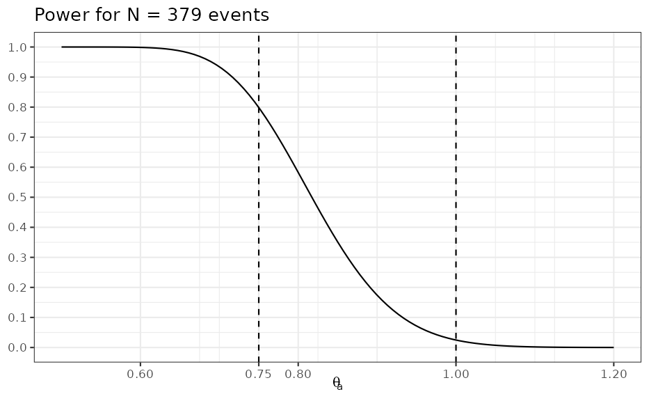

Critical value

The critical value determines at which observed logHR we just conclude that the success criterion is fulfilled.

design_crit <- decision1S_boundary(unit_inf, Nev, success_crit, sigma=2)

design_crit

## [1] -0.2017185

exp(design_crit)

## [1] 0.8173249

We can check this:

success_crit(postmix(unit_inf, m=design_crit, n=379))

## Using default prior reference scale 2

## [1] 1

Ok, when observing the critical value, we get a success.

Now, what if we observe a 1% worse result?

success_crit(postmix(unit_inf, m=design_crit+log(1.01), n=379))

## Using default prior reference scale 2

## [1] 0

No success then $\Rightarrow$ this is the critical boundary value.

PoS at interim for phase III trial A only

No use of historical information

Posterior of treatment effect at interim. The trial uses a non-informative prior for the treatment effect:

interim_A <- postmix(unit_inf, m=trials$logHR[3], se=trials$sem[3])
interim_A

## Univariate normal mixture
## Reference scale: 2
## Mixture Components:
##   comp1     
## w  1.0000000
## m -0.1851865
## s  0.1566521

Now we are interested in the PoS at trial completion. The prior to use for the analysis of the second half is given by the data collected so far.

interim_pos_A <- pos1S(interim_A, Nev-trials$deaths[3], success_crit, sigma=2)

The returned function can now calculate the PoS assuming any distribution on the treatment effect. In case we do not use any historical information, then this is just the interim posterior:

interim_pos_A(interim_A)

## [1] 0.4465623

The above command integrates the conditional power over the uncertainty which we have about the treatment effect as defined above for $PoS_I$ .

The conditional power and the operating characteristics of a trial coincide whenever we do not condition on any observed data. The key difference of the conditional power as compared to the probability of success is that it assumes a known value for the parameter of interest. This can be seen as follows: First define the conditional power which is conditional on the observed data, $CP_{N-n_I}(\theta|y_{n_I})$ :

interim_oc_A <- oc1S(interim_A, Nev-trials$deaths[3], success_crit, sigma=2)

The conditional power assuming the alternative is true (a HR of 0.75):

interim_oc_A(alt_logHR)

## [1] 0.708769

In case there is no uncertainty of the treatment effect (here $se=10^-4$ ), then this result agrees with the probability of success calculation:

interim_pos_A(mixnorm(c(1, alt_logHR, 1E-4)))

## [1] 0.7087689

For trial B the calculation is:

interim_B <- postmix(unit_inf, m=trials$logHR[4], se=trials$sem[4])
interim_pos_B <- pos1S(interim_B, Nev-trials$deaths[4], success_crit, sigma=2)
interim_pos_B(interim_B)

## [1] 0.6411569

Use of historical information - MAP approach

However, we have historical information of which we can take advantage at the interim for a better informed decision.

Our data before the phase III trials includes the PoC and the phase II trial. We now derive from these a MAP prior; recall that the MAP prior is the prediction of the log-hazard ratio of a future trial:

base <- trials[1:2,]

set.seed(342345)
base_map_mc <- gMAP(cbind(logHR, sem) ~ 1 | study,
                    family=gaussian,
                    data=base,
                    weights=deaths,
                    tau.dist="HalfNormal", tau.prior=0.5,
                    beta.prior=cbind(0, 2))

forest_plot(base_map_mc, est="MAP")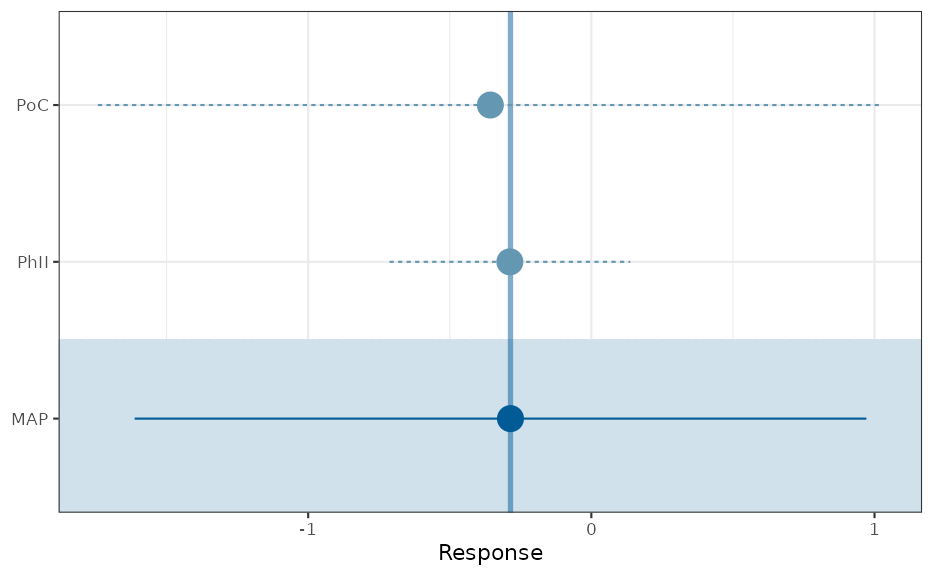

base_map <- automixfit(base_map_mc)

plot(base_map)$mix + xlab(expression(log(theta)))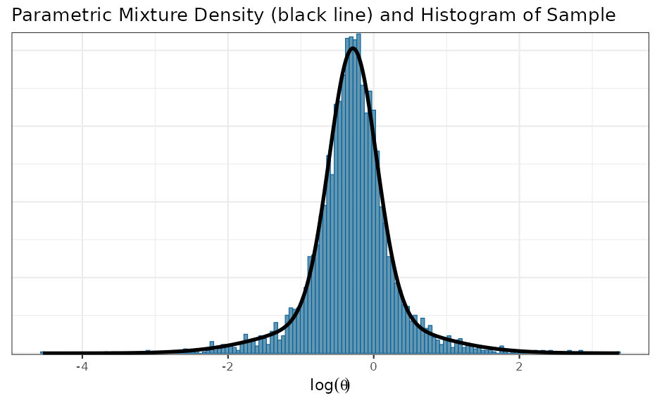

base_map

## EM for Normal Mixture Model
## Log-Likelihood = -3110.728
## 
## Univariate normal mixture
## Reference scale: 2
## Mixture Components:
##   comp1      comp2      comp3     
## w  0.6094510  0.2591800  0.1313691
## m -0.2943573 -0.2783962 -0.3331379
## s  0.2990546  0.6500315  1.1889177

At the interim we have even more knowledge available on the treatment effect through the interim data itself which we can include into the MAP prior:

interim_A_combined <- postmix(base_map, m=trials$logHR[3], se=trials$sem[3])

The PoS for this posterior at interim (representing historical and interim data collected) is:

interim_pos_A(interim_A_combined)

## [1] 0.4850564

Note that we have not redefined interim_pos_A, such that this calculates the PoS for the phase III A trial taking into account that the final analysis will use a non-informative prior.

For trial B the calculation is:

interim_B_combined <- postmix(base_map, m=trials$logHR[4], se=trials$sem[4])
interim_pos_B(interim_B_combined)

## [1] 0.6686476

Use of historical information - MAC approach

However, there is even more information which can be used here, since the phase III result of trial B is also available:

interim_map_mc <- update(base_map_mc, data=trials)

Now the trial B specific posterior at interim is

kable(fitted(interim_map_mc), digits=3)

	mean	sd	2.5%	50%	97.5%
PoC	-0.244	0.238	-0.795	-0.238	0.234
PhII	-0.252	0.149	-0.556	-0.251	0.042
PhIII_A	-0.214	0.126	-0.462	-0.216	0.035
PhIII_B	-0.237	0.126	-0.489	-0.237	0.011

which we can extract as:

obtain posterior (which we restrict to the first 4 columns)

interim_map_post <- as.matrix(interim_map_mc)[,1:4]

dim(interim_map_post) # posterior is given as matrix: iteration x parameter

## [1] 4000    4

head(interim_map_post, n=3)

##           parameters
## iterations   theta[1]   theta[2]   theta[3]    theta[4]
##       [1,]  0.5793535 -0.4054789  0.1303989 -0.30952085
##       [2,] -0.3457577 -0.3818282 -0.3105840 -0.32644175
##       [3,] -0.1232030 -0.1211176 -0.1414171 -0.08166256

turn MCMC posterior sample into parametric mixture

interim_A_allcombined <- automixfit(interim_map_post[,"theta[3]"])

and finally evaluate the PoS

interim_pos_A(interim_A_allcombined)

## [1] 0.5030811

which aligns with the published result under the assumption of full exchangeability.

For trial B computations are:

interim_B_allcombined <- automixfit(interim_map_post[,"theta[4]"])
interim_pos_B(interim_B_allcombined)

## [1] 0.6415822

Differential discounting

Differential discounting allows to weight different data-sources differently. For example, we may assume greater heterogeneity for the historical data in comparison to the twin phase III trials.

Assign data to historical (2) and concurrent data strata (1):

trials <- trials %>% mutate(stratum=c(2, 2, 1, 1))

kable(trials, digits=2)

study	deaths	HR	logHR	sem	stratum
PoC	8	0.70	-0.36	0.71	2
PhII	85	0.75	-0.29	0.22	2
PhIII_A	162	0.83	-0.19	0.16	1
PhIII_B	150	0.78	-0.25	0.16	1

set.seed(435345)
interim_diff_map_mc <- gMAP(cbind(logHR, sem) ~ 1 | study,
                            tau.strata=stratum,
                            family=gaussian,
                            data=trials,
                            weights=deaths,
                            tau.dist="HalfNormal", tau.prior=c(0.5, 1),
                            beta.prior=cbind(0, 2))

interim_diff_map_post <- as.matrix(interim_diff_map_mc)[,1:4]

interim_A_diff_allcombined <- automixfit(interim_diff_map_post[,"theta[3]"])
interim_B_diff_allcombined <- automixfit(interim_diff_map_post[,"theta[4]"])

interim_pos_A(interim_A_diff_allcombined)

## [1] 0.493427

interim_pos_B(interim_B_diff_allcombined)

## [1] 0.6394128

PoS for both phase III trials being successful

So far we have only calculated the individual PoS per trial, but more interesting is the overall PoS for both trials being successful.

Recall, the PoS is the conditional power integrated over an assumed true effect distribution. Hence, we had for trial A:

interim_pos_A(interim_A)

## [1] 0.4465623

As explained, the conditional power is the operating characerstic of a design when conditioning on the already observed data:

interim_oc_A <- oc1S(interim_A, Nev-trials$deaths[3], success_crit, sigma=2)

The PoS is then the integral of the conditional power over the parameter space $\theta$ representing our knowledge. This integral can be evaluated in a Monte-Carlo (MC) approach as

$PoS_I = \int CP_{N-n_I}(\theta|y_{n_I}) \, p(\theta|y_{n_I}) \, d\theta \approx \frac{1}{S} \sum_{i=1}^S CP(\theta_i),$

whenever we have a sample of $p(\theta|y_{n_I})$ of size $S$ … which we have:

interim_A_samp <- rmix(interim_A, 1E4)
mean(interim_oc_A(interim_A_samp))

## [1] 0.4479449

This is an MC approach to calculating the PoS.

When now considering the probability for both trials being successful we have to perform an MC integration over the joint density $p(\theta_A,\theta_B|y_{n_{I_A}},y_{n_{I_B}})$

$\begin{aligned} PoS &= \iint CP_{N-n_{I_A}}(\theta_A|y_{n_{I_A}}) \, CP_{N-n_{I_B}}(\theta_B|y_{n_{I_B}})\, p(\theta_A,\theta_B|y_{n_{I_A}},y_{n_{I_B}}) \, d\theta_A d\theta_B \\ & \approx \frac{1}{S} \sum_{i=1}^S CP_{N-n_{I_A}}(\theta_{A,i}|y_{n_{I_A}}) \, CP_{N-n_{I_B}}(\theta_{B,i}|y_{n_{I_B}}). \end{aligned}$

Thus we need to also get the conditional power for trial B at interim…

interim_oc_B <- oc1S(interim_B, Nev-trials$deaths[4], success_crit, sigma=2)

…and integrate over the posterior samples (differential discounting case)

mean(interim_oc_A(interim_diff_map_post[,"theta[3]"]) * interim_oc_B(interim_diff_map_post[,"theta[4]"]))

## [1] 0.3452887

which is slightly larger than assuming independence:

interim_pos_A(interim_A) * interim_pos_B(interim_B)

## [1] 0.2863165

This is due to dependence of the posteriors

cor(interim_diff_map_post[,c("theta[3]", "theta[4]")])

##           theta[3]  theta[4]
## theta[3] 1.0000000 0.3187079
## theta[4] 0.3187079 1.0000000

For the full exchangeability case we have

mean(interim_oc_A(interim_map_post[,"theta[3]"]) * interim_oc_B(interim_map_post[,"theta[4]"]))

## [1] 0.3521087

Summary

We have now calculated with increasing complexity the probability of success for various data constellations. As new trials are only conducted whenever previous trial results were positive, it is important to take note of the potential selection bias. Moreover, adding more historical data sources in this situation will likely increase the probability of success as illustrated by this summary of our preceding calculations.

Phase III trial A:

## only interim data of trial A 
interim_pos_A(interim_A)

## [1] 0.4465623

## in addition with prior historical data PoC & phase II data
interim_pos_A(interim_A_combined)

## [1] 0.4850564

## finally with the interim data of the phase III B
interim_pos_A(interim_A_allcombined)

## [1] 0.5030811

Phase III trial B:

## only interim data of trial B
interim_pos_B(interim_B)

## [1] 0.6411569

## in addition with prior historical data PoC & phase II data
interim_pos_B(interim_B_combined)

## [1] 0.6686476

## finally with the interim data of the phase III A
interim_pos_B(interim_B_allcombined)

## [1] 0.6415822

Appendix: MAP and MAC equivalence

In the preceeding sections we have used MAP and MAC equivalence already. The proof for the equivalence is presented reference in [2]. The formal deriavtion is shown at the end of this section

While MAP and MAC provide the exact same results, the difference is a sequential vs a joint analysis as (see also [2]):

MAP: Summarize historical information as MAP and then update the MAP with the trial result (MCMC, then postmix).
MAC: Directly summarize historical information and trial result in a single step (only MCMC on all data).

The two results above using MAP and MAC did not line up. The reason here is that the MAP approach used the historical data and the phase III trial A interim data only. In contrast, the MAC approach used the historical data and interim phase III data of both trials. To show the equivalence we need to align this mismatch of used data.

Run gMAP with base data and produce a large MCMC sample (10 chains) to get a very high precision.

base_map_mc_2 <- gMAP(cbind(logHR, sem) ~ 1 | study,
                      family=gaussian,
                      data=base,
                      weights=deaths,
                      tau.dist="HalfNormal", tau.prior=0.5,
                      beta.prior=cbind(0, 2),
                      chains=ifelse(is_CRAN, 2, 20))

Force an accurate fit with 5 components:

base_map_2 <- mixfit(base_map_mc_2, Nc=5)
base_map_2

## EM for Normal Mixture Model
## Log-Likelihood = -15088.42
## 
## Univariate normal mixture
## Reference scale: 2
## Mixture Components:
##   comp1       comp2       comp3       comp4       comp5      
## w  0.40929935  0.20586574  0.18866513  0.12833707  0.06783271
## m -0.28173830 -0.64782890  0.06087094  0.16129924 -1.05921673
## s  0.22707579  0.32358363  0.33140706  0.86765455  0.73553054

Now, combine the MAP prior (representing historical knowledge) with the interim data of trial A:

interim_A_combined_2 <- postmix(base_map_2, m=trials$logHR[3], se=trials$sem[3])

Run the respective MAC analysis (thus we need historical data + phase III A trial, but excluding the phase III B data):

interim_map_mc_2 <- update(base_map_mc_2, data=trials[-4,])

## Warning: There were 3 divergent transitions after warmup. See
## https://mc-stan.org/misc/warnings.html#divergent-transitions-after-warmup
## to find out why this is a problem and how to eliminate them.

## Warning: Examine the pairs() plot to diagnose sampling problems

## Warning in gMAP(formula = cbind(logHR, sem) ~ 1 | study, family = gaussian, : In total 3 divergent transitions occured during the sampling phase.
## Please consider increasing adapt_delta closer to 1 with the following command prior to gMAP:
## options(RBesT.MC.control=list(adapt_delta=0.999))

interim_map_post_2 <- as.matrix(interim_map_mc_2)[,1:3]

turn MCMC posterior sample into parametric mixture

interim_A_allcombined_2 <- mixfit(interim_map_post_2[,"theta[3]"], Nc=5)

interim_A_allcombined_2

## EM for Normal Mixture Model
## Log-Likelihood = 10763.73
## 
## Univariate normal mixture
## Mixture Components:
##   comp1       comp2       comp3       comp4       comp5      
## w  0.22608509  0.22287087  0.22104424  0.19134605  0.13865375
## m -0.22358073 -0.31478209 -0.11546035 -0.32415990 -0.01378153
## s  0.05767847  0.12976158  0.06117267  0.07871764  0.09025686

Now let’s overlay the two posterior’s

ggplot(data.frame(logHR=c(-0.8,0.25)), aes(logHR)) +
    stat_function(fun=dmix, args=list(mix=interim_A_combined_2), aes(linetype="MAP")) +
    stat_function(fun=dmix, args=list(mix=interim_A_allcombined_2), aes(linetype="MAC")) +
    scale_linetype_discrete("Analysis") +
    ggtitle("Posterior log hazard of phase III A trial at interim")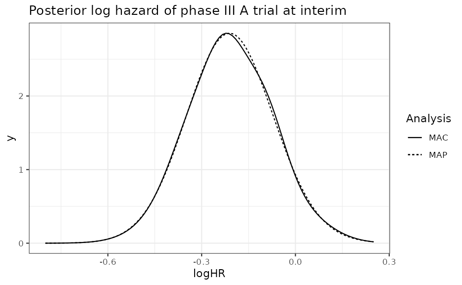

The PoS is essentially the same

interim_pos_A(interim_A_combined_2)

## [1] 0.489214

interim_pos_A(interim_A_allcombined_2)

## [1] 0.4943454

Formal MAP and MAC equivalence

The stated equivalence requires that the posterior of a trial specific parameter

$p(\theta_\star|y_\star,y_H),$

which is conditional on the trial specific data $y_\star$ and the historical data $y_H$ (MAC approach, joint use of $y_H,y_\star$ ), is equivalent to obtaining the MAP prior $p(\theta_\star|y_H)$ based on the historical data and then analyzing the new trial with this prior.

$\begin{aligned} p(\theta_\star|y_\star,y_H) &\propto p(\theta_\star,\theta_H|y_\star,y_H) \\ &\propto p(y_\star,y_H|\theta_\star,\theta_H) \, p(\theta_\star,\theta_H) \\ &= p(y_\star|\theta_\star) \, p(y_H|\theta_H) \, p(\theta_\star,\theta_H) \\ &\propto p(y_\star|\theta_\star) \, p(\theta_\star,\theta_H|y_H) \\ &\propto p(y_\star|\theta_\star) \, p(\theta_\star|y_H) \end{aligned}$

The equivalence holds under the use of the meta-analytic model.

References

[1] Neuenschwander, B., Roychoudhury, S., & Schmidli, H. (2016). On the Use of Co-Data in Clinical Trials. Statistics in Biopharmaceutical Research, 8(3), 345-354.

[2] 1. Schmidli H, Gsteiger S, Roychoudhury S, O’Hagan A, Spiegelhalter D, Neuenschwander B. Robust meta-analytic-predictive priors in clinical trials with historical control information. Biometrics. 2014;70(4):1023-1032.

R Session Info

sessionInfo()

## R version 4.4.2 (2024-10-31)
## Platform: x86_64-pc-linux-gnu
## Running under: Ubuntu 22.04.5 LTS
## 
## Matrix products: default
## BLAS:   /usr/lib/x86_64-linux-gnu/openblas-pthread/libblas.so.3 
## LAPACK: /usr/lib/x86_64-linux-gnu/openblas-pthread/libopenblasp-r0.3.20.so;  LAPACK version 3.10.0
## 
## locale:
##  [1] LC_CTYPE=C.UTF-8       LC_NUMERIC=C           LC_TIME=C.UTF-8       
##  [4] LC_COLLATE=C.UTF-8     LC_MONETARY=C.UTF-8    LC_MESSAGES=C.UTF-8   
##  [7] LC_PAPER=C.UTF-8       LC_NAME=C              LC_ADDRESS=C          
## [10] LC_TELEPHONE=C         LC_MEASUREMENT=C.UTF-8 LC_IDENTIFICATION=C   
## 
## time zone: UTC
## tzcode source: system (glibc)
## 
## attached base packages:
## [1] stats     graphics  grDevices utils     datasets  methods   base     
## 
## other attached packages:
## [1] purrr_1.0.2      dplyr_1.1.4      bayesplot_1.11.1 ggplot2_3.5.1   
## [5] knitr_1.49       RBesT_1.7-4     
## 
## loaded via a namespace (and not attached):
##  [1] gtable_0.3.6         tensorA_0.36.2.1     xfun_0.49           
##  [4] bslib_0.8.0          QuickJSR_1.4.0       htmlwidgets_1.6.4   
##  [7] inline_0.3.20        vctrs_0.6.5          tools_4.4.2         
## [10] generics_0.1.3       stats4_4.4.2         parallel_4.4.2      
## [13] tibble_3.2.1         fansi_1.0.6          pkgconfig_2.0.3     
## [16] checkmate_2.3.2      desc_1.4.3           distributional_0.5.0
## [19] RcppParallel_5.1.9   assertthat_0.2.1     lifecycle_1.0.4     
## [22] compiler_4.4.2       farver_2.1.2         stringr_1.5.1       
## [25] textshaping_0.4.0    munsell_0.5.1        codetools_0.2-20    
## [28] htmltools_0.5.8.1    sass_0.4.9           yaml_2.3.10         
## [31] Formula_1.2-5        pillar_1.9.0         pkgdown_2.1.1       
## [34] jquerylib_0.1.4      cachem_1.1.0         StanHeaders_2.32.10 
## [37] abind_1.4-8          posterior_1.6.0      rstan_2.32.6        
## [40] tidyselect_1.2.1     digest_0.6.37        stringi_1.8.4       
## [43] mvtnorm_1.3-2        reshape2_1.4.4       labeling_0.4.3      
## [46] fastmap_1.2.0        grid_4.4.2           colorspace_2.1-1    
## [49] cli_3.6.3            magrittr_2.0.3       loo_2.8.0           
## [52] pkgbuild_1.4.5       utf8_1.2.4           withr_3.0.2         
## [55] scales_1.3.0         backports_1.5.0      rmarkdown_2.29      
## [58] matrixStats_1.4.1    gridExtra_2.3        ragg_1.3.3          
## [61] evaluate_1.0.1       rstantools_2.4.0     rlang_1.1.4         
## [64] Rcpp_1.0.13-1        glue_1.8.0           jsonlite_1.8.9      
## [67] R6_2.5.1             plyr_1.8.9           systemfonts_1.1.0   
## [70] fs_1.6.5

Use of Co-Data in Clinical Trails with RBesT

Sebastian Weber

2024-11-21