Mixture Distributions

Density, cumulative distribution function, quantile function and random number generation for supported mixture distributions. (d/p/q/r)mix are generic and work with any mixture supported by BesT (see table below).

Usage

dmix(mix, x, log = FALSE)

pmix(mix, q, lower.tail = TRUE, log.p = FALSE)

qmix(mix, p, lower.tail = TRUE, log.p = FALSE)

rmix(mix, n)

# S3 method for mix
[[(mix, ..., rescale = FALSE)

Arguments

mix: mixture distribution object
x, q: vector of quantiles
log, log.p: logical; if TRUE (not default), probabilities $p$ are given as $\log(p)$
lower.tail: logical; if TRUE (default), probabilities are $P[X\leq x]$ otherwise, $P[X>x]$
p: vector of probabilities
n: number of observations. If length(n) > 1, the length is taken to be the number required
...: components to subset given mixture.
rescale: logical; if TRUE, mixture weights will be rescaled to sum to 1

Value

dmix gives the weighted sum of the densities of each component.

pmix calculates the distribution function by evaluating the weighted sum of each components distribution function.

qmix returns the quantile for the given p

by using that the distribution function is monotonous and hence a gradient based minimization scheme can be used to find the matching quantile q.

rmix generates a random sample of size n by first sampling a latent component indicator in the range $1..K$ for each draw and then the function samples from each component a random draw using the respective sampling function. The rnorm function returns the random draws as numerical vector with an additional attribute ind which gives the sampled component indicator.

Details

A mixture distribution is defined as a linear superposition of $K$ densities of the same distributional class. The mixture distributions supported have the form

$$f(x,\mathbf{w},\mathbf{a},\mathbf{b}) = \sum_{k=1}^K w_k \, f_k(x,a_k,b_k).$$

The $w_k$ are the mixing coefficients which must sum to $1$. Moreover, each density $f$ is assumed to be parametrized by two parameters such that each component $k$ is defined by a triplet, $(w_k,a_k,b_k)$.

Individual mixture components can be extracted using the [[ operator, see examples below.

The supported densities are normal, beta and gamma which can be instantiated with mixnorm, mixbeta, or mixgamma, respectively. In addition, the respective predictive distributions are supported. These can be obtained by calling preddist which returns appropriate normal, beta-binomial or Poisson-gamma mixtures.

For convenience a summary function is defined for all mixtures. It returns the mean, standard deviation and the requested quantiles which can be specified with the argument probs.

Supported Conjugate Prior-Likelihood Pairs

Prior/Posterior	Likelihood	Predictive	Summaries
Beta	Binomial	Beta-Binomial	`n`, `r`
Normal	Normal (fixed $\sigma$)	Normal	`n`, `m`, `se`
Gamma	Poisson	Gamma-Poisson	`n`, `m`
Gamma	Exponential	Gamma-Exp (not supported)	`n`, `m`

Examples

## a beta mixture
bm <- mixbeta(weak=c(0.2, 2, 10), inf=c(0.4, 10, 100), inf2=c(0.4, 30, 80))

## extract the two most informative components
bm[[c(2,3)]]
#> Univariate beta mixture
#> Mixture Components:
#>   inf   inf2 
#> w   0.4   0.4
#> a  10.0  30.0
#> b 100.0  80.0
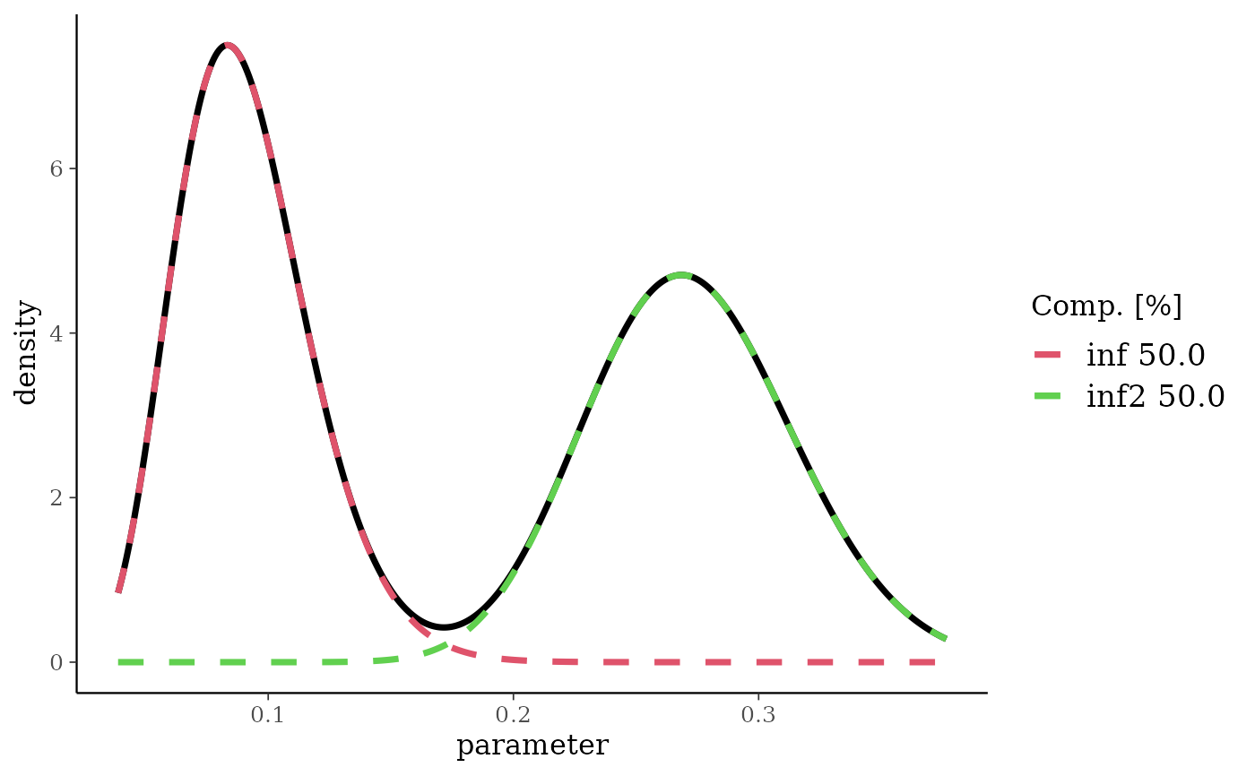
## rescaling needed in order to plot
plot(bm[[c(2,3),rescale=TRUE]])


summary(bm)
#>       mean         sd       2.5%      50.0%      97.5% 
#> 0.17878788 0.09898301 0.04389723 0.15654866 0.35327791