Fit of Mixture Densities to Samples

Expectation-Maximization (EM) based fitting of parametric mixture densities to numerical samples. This provides a convenient approach to approximate MCMC samples with a parametric mixture distribution.

Usage

mixfit(sample, type = c("norm", "beta", "gamma", "mvnorm"), thin, ...)

# Default S3 method
mixfit(sample, type = c("norm", "beta", "gamma", "mvnorm"), thin, ...)

# S3 method for class 'gMAP'
mixfit(sample, type, thin, ...)

# S3 method for class 'gMAPpred'
mixfit(sample, type, thin, ...)

# S3 method for class 'array'
mixfit(sample, type, thin, ...)

Arguments

sample: Sample to be fitted.
type: Mixture density to use. Can be either norm, beta or gamma.
thin: Thinning applied to the sample. See description for default behavior.
...: Parameters passed to the low-level EM fitting functions. Parameter Nc is mandatory.

Value

A mixture object according the requested type is returned. The object has additional information attached, i.e. the log-likelihood can be queried and diagnostic plots can be generated. See links below.

Details

Parameters of EM fitting functions

Nc: Number of mixture components. Required parameter.
mix_init: Initial mixture density. If missing (default) then a k-nearest-neighbor algorithm is used to find an initial mixture density.
Ninit: Number of data points used for initialization. Defaults to 50.
verbose: If set to TRUE the function will inform about fitting process
maxIter: Maximal number of iterations. Defaults to 500.
tol: Defines a convergence criteria as an upper bound for the change in the log-likelihood, i.e. once the derivative (with respect to iterations) of the log-likelihood falls below tol, the function declares convergence and stops.
eps: Must be a triplet of numbers which set the desired accuracy of the inferred parameters per mixture component. See below for a description of the parameters used during EM. EM is stopped once a running mean of the absolute difference between the last successive Neps estimates is below the given eps for all parameters. Defaults to 5E-3 for each parameter.
Neps: Number of iterations used for the running mean of parameter estimates to test for convergence. Defaults to 5.
constrain_gt1: Logical value controlling if the Beta EM constrains all parameters a & b to be greater than 1. By default constraints are turned on (new since 1.6-0).

By default the EM convergence is declared when the desired accuracy of the parameters has been reached over the last Neps estimates. If tol and Neps is specified, then whatever criterion is met first will stop the EM.

The parameters per component \(k\) used internally during fitting are for the different EM procedures:

normal: \(logit(w_k), \mu_k, \log(\sigma_k)\)
beta: \(logit(w_k), \log(a_k), \log(b_k)\)
constrained beta: \(logit(w_k), \log(a_k-1), \log(b_k-1)\)
gamma: \(logit(w_k), \log(\alpha_k), \log(\beta_k)\)

Note: Whenever no mix_init argument is given, the EM fitting routines assume that the data vector is given in random order. If in the unlikely event that the EM gets caught in a local extremum, then random reordering of the data vector may alleviate the issue.

Methods (by class)

mixfit(default): Performs an EM fit for the given sample. Thinning is applied only if thin is specified.
mixfit(gMAP): Fits the default predictive distribution from a gMAP analysis. Automatically obtains the predictive distribution of the intercept only case on the response scale mixture from the gMAP object. For the binomial case a beta mixture, for the gaussian case a normal mixture and for the Poisson case a gamma mixture will be used. In the gaussian case, the resulting normal mixture will set the reference scale to the estimated sigma in gMAP call.
mixfit(gMAPpred): Fits a mixture density for each prediction from the gMAP prediction.
mixfit(array): Fits a mixture density for an MCMC sample. It is recommended to provide a thinning argument which roughly yields independent draws (i.e. use acf to identify a thinning lag with small auto-correlation). The input array is expected to have 3 dimensions which are nested as iterations, chains, and draws.

References

Dempster A.P., Laird N.M., Rubin D.B. Maximum Likelihood from Incomplete Data via the EM Algorithm. Journal of the Royal Statistical Society, Series B 1977; 39 (1): 1-38.

Examples

bmix <- mixbeta(rob=c(0.2, 1, 1), inf=c(0.8, 10, 2))

bsamp <- rmix(bmix, 1000)

bfit <- mixfit(bsamp, type="beta", Nc=2)

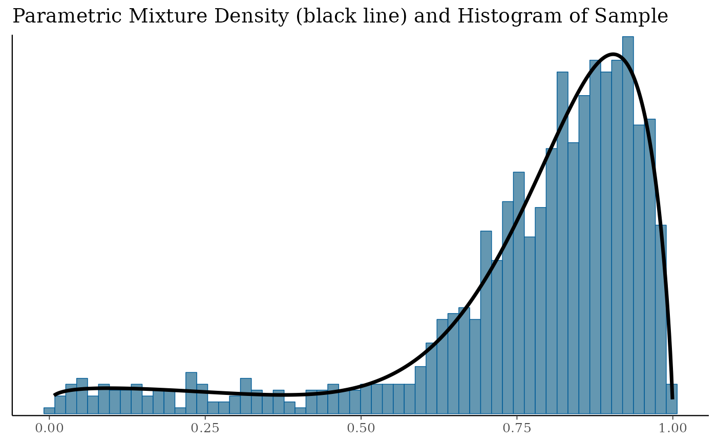
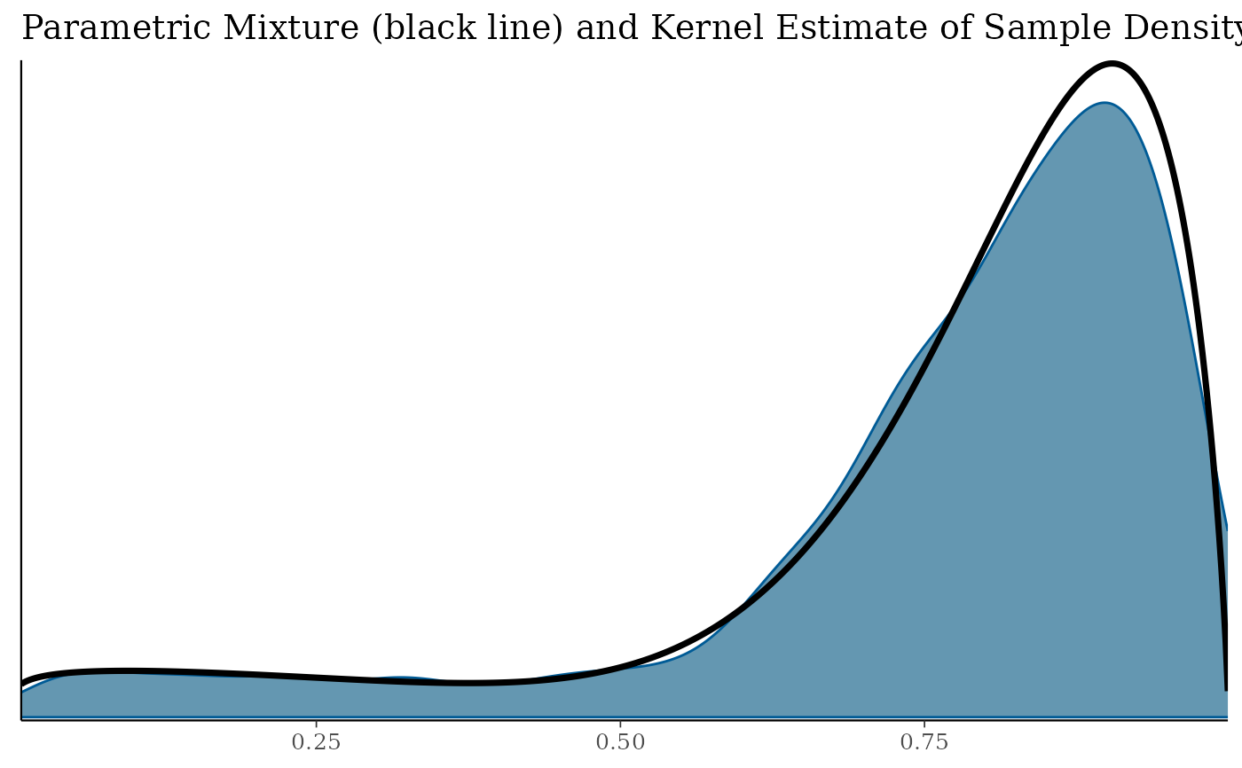
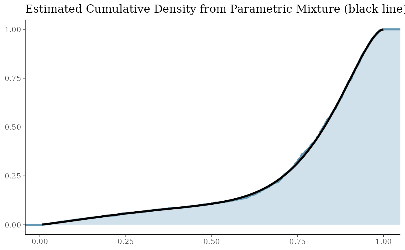
# diagnostic plots can easily by generated from the EM fit with
bfit.check <- plot(bfit)

names(bfit.check)
#> [1] "mixdist" "mixdens" "mixecdf" "mix"    

# check convergence of parameters
bfit.check$mix

bfit.check$mixdens

bfit.check$mixecdf


# obtain the log-likelihood
logLik(bfit)
#> 'log Lik.' 543.9702 (df=5)

# or AIC
AIC(bfit)
#> [1] -1077.94