Normal Mixture Density

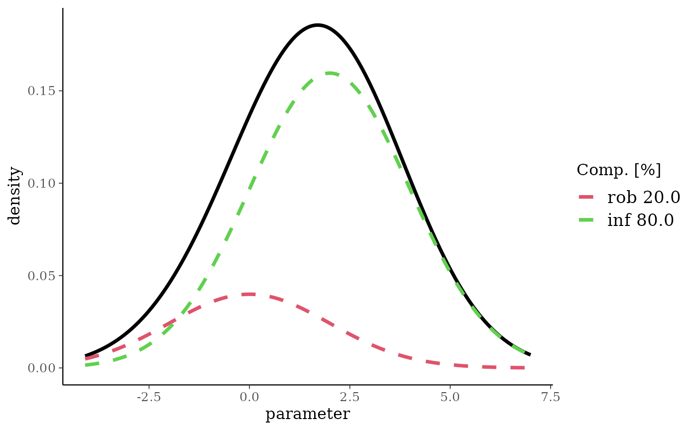
The normal mixture density and auxiliary functions.

Usage

mixnorm(..., sigma, param = c("ms", "mn"))

mn2norm(m, n, sigma, drop = TRUE)

# S3 method for class 'normMix'
print(x, ...)

# S3 method for class 'normMix'
summary(object, probs = c(0.025, 0.5, 0.975), ...)

# S3 method for class 'normMix'
sigma(object, ...)

sigma(object) <- value

Arguments

...: List of mixture components.
sigma: Reference scale.
param: Determines how the parameters in the list are interpreted. See details.
m: Vector of means
n: Vector of sample sizes.
drop: Delete the dimensions of an array which have only one level.
x: The mixture to print
object: Normal mixture object.
probs: Quantiles reported by the summary function.
value: New value of the reference scale sigma.

Value

Returns a normal mixture with the specified mixture components. mn2norm returns the mean and standard deviation given a mean and sample size parametrization.

Details

Each entry in the ... argument list is expected to be a triplet of numbers which defines the weight \(w_k\), first and second parameter of the mixture component \(k\). A triplet can optionally be named which will be used appropriately.

The first and second parameter can be given in different parametrizations which is set by the param option:

ms: Mean and standard deviation. Default.
mn: Mean and number of observations. n determines s via the relation \(s=\sigma/\sqrt{n}\) with \(\sigma\) being the fixed reference scale.

The reference scale \(\sigma\) is the fixed standard deviation in the one-parameter normal-normal model (observation standard deviation). The function sigma can be used to query the reference scale and may also be used to assign a new reference scale, see examples below. In case the sigma is not specified, the user has to supply sigma as argument to functions which require a reference scale.

Functions

sigma(object) <- value: Allows to assign a new reference scale sigma.

Examples


nm <- mixnorm(rob=c(0.2, 0, 2), inf=c(0.8, 2, 2), sigma=5)

print(nm)
#> Univariate normal mixture
#> Reference scale: 5
#> Mixture Components:
#>   rob inf
#> w 0.2 0.8
#> m 0.0 2.0
#> s 2.0 2.0
summary(nm)
#>      mean        sd      2.5%     50.0%     97.5% 
#>  1.600000  2.154066 -2.708104  1.631171  5.740143 
plot(nm)


set.seed(57845)
mixSamp <- rmix(nm, 500)
plot(nm, samp=mixSamp)


# support defined by quantiles
qmix(nm, c(0.01, 0.99))
#> [1] -3.532815  6.491874

# density function
dmix(nm, seq(-5,5,by=2))
#> [1] 0.002101903 0.019963080 0.087013571 0.176032663 0.153777890 0.053559868

# distribution function
pmix(nm, seq(-5,5,by=2))
#> [1] 0.001428036 0.018329173 0.115153269 0.385122523 0.739808529 0.945312306

# the reference scale can be changed (it determines the ESS)
ess(nm)
#> Using default prior reference scale 5
#> [1] 5.404787

sigma(nm) <- 10
ess(nm)
#> Using default prior reference scale 10
#> [1] 21.61915