Plot mixture distributions

Plotting for mixture distributions

Usage

# S3 method for class 'mix'
plot(x, prob = 0.99, fun = dmix, log = FALSE, comp = TRUE, size = 1.25, ...)

# S3 method for class 'mvnormMix'
plot(x, prob = 0.99, fun = dmix, log = FALSE, comp = TRUE, size = 1.25, ...)

Arguments

x

mixture distribution

prob

defining lower and upper percentile of x-axis. Defaults to the 99% central probability mass.

fun

function to plot which can be any of dmix, qmix or pmix.

log

log argument passed to the function specified in fun.

comp

for the density function this can be set to TRUE which will display colour-coded each mixture component of the density in addition to the density.

size

controls the linesize in plots.

...

extra arguments passed on to the plotted function.

Value

A ggplot object is returned.

Details

Plot function for mixture distribution objects. It shows the density/quantile/cumulative distribution (corresponds to d/q/pmix function) for some specific central probability mass defined by prob. By default the x-axis is chosen to show 99% of the probability density mass.

Customizing ggplot2 plots

The returned plot is a ggplot2 object. Please refer to the "Customizing Plots" vignette which is part of RBesT documentation for an introduction. For simple modifications (change labels, add reference lines, ...) consider the commands found in bayesplot-helpers. For more advanced customizations please use the ggplot2 package directly. A description of the most common tasks can be found in the R Cookbook and a full reference of available commands can be found at the ggplot2 documentation site.

See also

Other mixdist: mix, mixbeta(), mixcombine(), mixgamma(), mixmvnorm(), mixnorm()

Examples

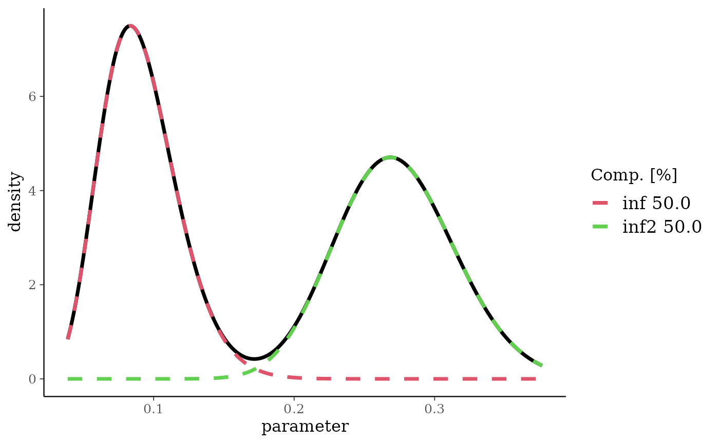
# beta with two informative components
bm <- mixbeta(inf=c(0.5, 10, 100), inf2=c(0.5, 30, 80))
plot(bm)

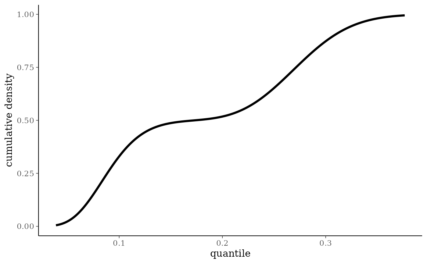
plot(bm, fun=pmix)


# for customizations of the plot we need to load ggplot2 first
library(ggplot2)

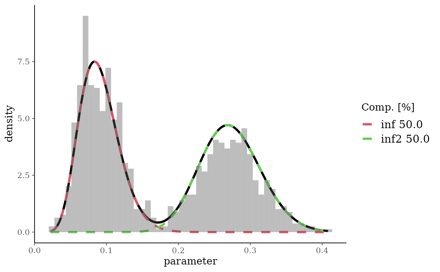
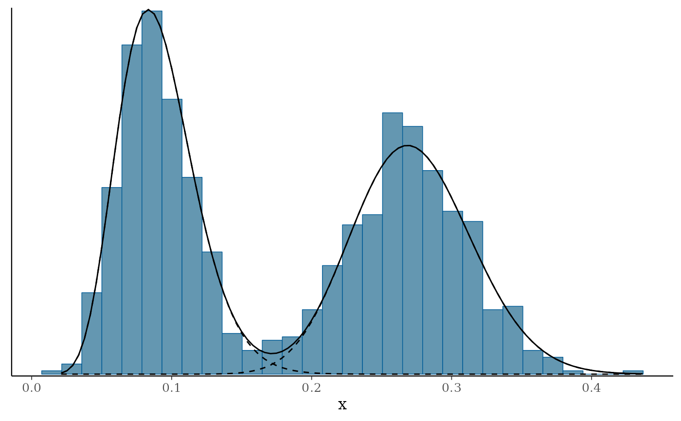
# show a histogram along with the density
plot(bm) + geom_histogram(data=data.frame(x=rmix(bm, 1000)),
                          aes(y=..density..), bins=50, alpha=0.4)
#> Warning: The dot-dot notation (`..density..`) was deprecated in ggplot2 3.4.0.
#> ℹ Please use `after_stat(density)` instead.
#> ℹ The deprecated feature was likely used in the RBesT package.
#>   Please report the issue at <https://github.com/Novartis/RBesT/issues>.


# \donttest{
# note: we can also use bayesplot for histogram plots with a density ...
library(bayesplot)
mh <- mcmc_hist(data.frame(x=rmix(bm, 1000)), freq=FALSE) +
         overlay_function(fun=dmix, args=list(mix=bm))
# ...and even add each component
for(k in 1:ncol(bm))
  mh <- mh + overlay_function(fun=dmix, args=list(mix=bm[[k]]), linetype=I(2))
print(mh)
#> `stat_bin()` using `bins = 30`. Pick better value with `binwidth`.

# }

# normal mixture
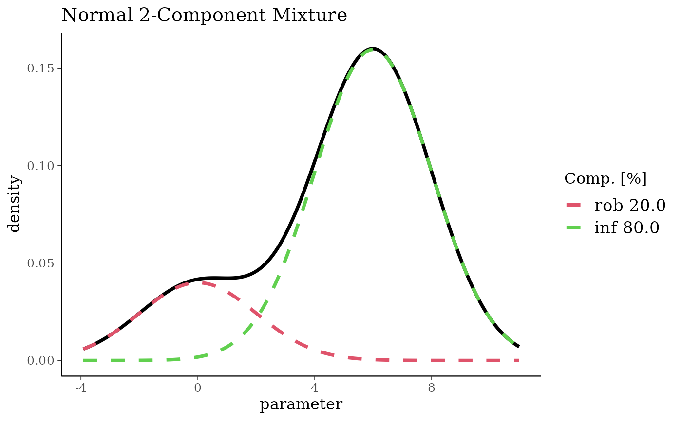
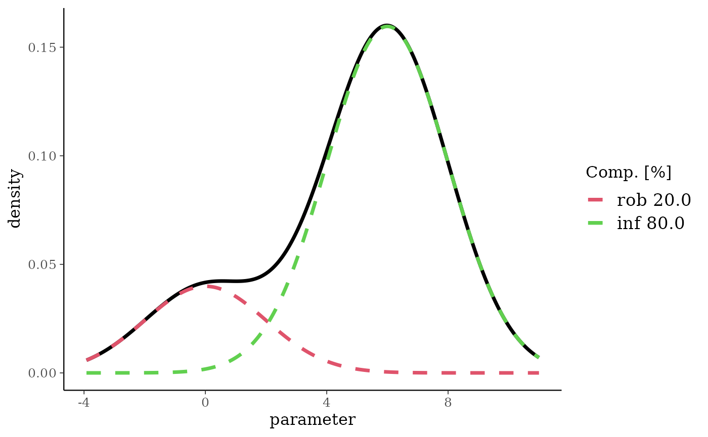
nm <- mixnorm(rob=c(0.2, 0, 2), inf=c(0.8, 6, 2), sigma=5)
plot(nm)

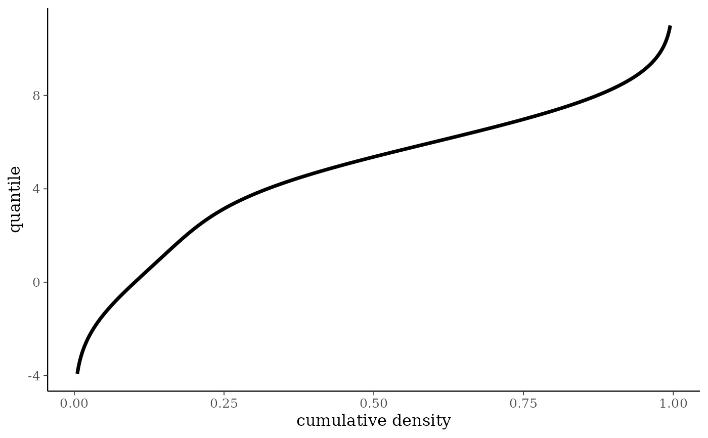
plot(nm, fun=qmix)


# obtain ggplot2 object and change title
pl <- plot(nm)
pl + ggtitle("Normal 2-Component Mixture")