PK - Multiple Ascending Dose - Using Novartis dzz file

Overview

This document contains PK exploratory graphs and also the R code that generates these graphs, starting from the dzz and PPtmp files that are stored here:

Data specifications can be accessed on Datasets and Rmarkdown template to generate this page can be found on Rmarkdown-Template.

Setup

#clear variables and plots
  rm(list=ls()) #clear all variables except Task00.start.time
  
#set seed
  set.seed(123456)

#user name  
  user = Sys.getenv("USER")
  
## Ensure that no library from the user home will be loaded such that
## we run with the production packages only
 .libPaths(grep("home", .libPaths(), value=TRUE, invert=TRUE))
 .libPaths(grep("usr", .libPaths(), value=TRUE, invert=TRUE))
 
# add localLib to libPaths for locally installed packages
.libPaths(c("localLib", .libPaths()))

# will load from first filepath first, then look in .libPaths for more packages not in first path
# version matches package in first filepath, in the case of multiple instances of a package

  
#add key packages
  library(ggplot2)
  library(grid)
  library(gridExtra)
  library(tidyr)
  library(dplyr)
  library(lubridate)

#ggplot settings
  theme_set(theme_bw(base_size=12))
  
#xgx functions
  source("../R/xgx_packages_functions.R")

Load in data from dzz (concentrations) and format for plotting

LOQassay = 1
drug1 = "ABC123"
drug2 = "DEF456"
  
#load data located here:
d = read.csv("../Data/dzz_PKConc.csv",stringsAsFactors = FALSE)

#create columns with dosing regimen information, based on ARM
d = d %>%
  mutate(DOSSTR          = stringr::str_replace(ARM,"Phase Ib? ",""),
         DRG1STR         = stringr::str_replace(DOSSTR,paste0(drug1," "),""),
         DRG1STR         = stringr::str_extract(DRG1STR,"^\\d* *mg Q\\dW"),
         DRG1DOS0        = as.numeric(stringr::str_extract(DRG1STR,"\\d*")),
         DRG1REG          = stringr::str_extract(DRG1STR,"Q\\dW"),
         DRG2STR          = stringr::str_extract(DOSSTR,paste0(drug2," \\d* *mg Q\\dW")),
         DRG2STR          = stringr::str_replace(DRG2STR,paste0(drug2," "),""),
         DRG2DOS0         = as.numeric(stringr::str_extract(DRG2STR,"\\d*")),
         DRG2REG          = stringr::str_extract(DRG2STR,"Q\\dW"),
         Comed           = ifelse(is.na(DRG2DOS0),"monotherapy","combination"),
         DRG1.DRG2       = paste(DRG1DOS0,Comed))

#create columns with time and normalized PK
d = d %>%
  filter(PCDTC!="") %>%
  group_by(SUBJID) %>%
  mutate(CYCLE      = as.numeric(substr(VISIT,7,8)),
         NOMTIMEH   = (CYCLE-1)*28*24+TMTPT,
         DATE       = ymd_hms(PCDTC),
         DATE0      = ymd_hms(first(PCDTC)),
         TIMEH      = (DATE-DATE0)/3600,
         RESN       = as.numeric(RESN),
         CENS       = RESN<LOQassay,
         RESN       = ifelse(CENS,LOQassay,RESN),
         RESNorm    = RESN/DRG1DOS0) %>%
  ungroup() %>%
  filter(NOMTIMEH>0)

#create simplified column names for plotting
d = d %>%
  arrange(DRG1DOS0,desc(DRG1REG)) %>%
  mutate(ID = SUBJID,
         DOSElabel = factor(DRG1STR,levels=rev(unique(DRG1STR))), #for proper ordering
         DOSE0 = DRG1DOS0,
         DOSE0label = paste(DOSE0,"mg"),
         DOSE0label = factor(DOSE0label,levels=rev(unique(DOSE0label))),
         REG = DRG1REG,
         NOMTIME = NOMTIMEH,
         TIME = TIMEH,
         CONC=RESN,
         CONCnorm = RESNorm)

Load in data from PPtmp (NCA) and format for plotting

nca = read.csv("../Data/PPtmp_NCA.csv",stringsAsFactors = FALSE)

#create columns with dosing regimen information, based on ARM
nca = nca %>%
  mutate(DOSSTR          = stringr::str_replace(ARM,"Phase Ib? ",""),
         DRG1STR         = stringr::str_replace(DOSSTR,paste0(drug1," "),""),
         DRG1STR         = stringr::str_extract(DRG1STR,"^\\d* *mg Q\\dW"),
         DRG1DOS0        = as.numeric(stringr::str_extract(DRG1STR,"\\d*")),
         DRG1REG          = stringr::str_extract(DRG1STR,"Q\\dW"),
         DRG2STR          = stringr::str_extract(DOSSTR,paste0(drug2," \\d* *mg Q\\dW")),
         DRG2STR          = stringr::str_replace(DRG2STR,paste0(drug2," "),""),
         DRG2DOS0         = as.numeric(stringr::str_extract(DRG2STR,"\\d*")),
         DRG2REG          = stringr::str_extract(DRG2STR,"Q\\dW"),
         Comed           = ifelse(is.na(DRG2DOS0),"monotherapy","combination"),
         DRG1.DRG2       = paste(DRG1DOS0,Comed),
         PPORRESNnorm    = PPORRESN/DRG1DOS0)

#create simplified column names  
nca = nca %>%
  arrange(DRG1DOS0,desc(DRG1REG)) %>%
  mutate(ID = SUBJID,
         DOSElabel = factor(DRG1STR,levels=unique(DRG1STR)), #for proper ordering
         DOSE0 = DRG1DOS0,
         REG = DRG1REG)

Provide an overview of the data

Concentration over time, faceted by regimen, colored by dose

gg = ggplot(data = d, aes(x = NOMTIME, y = CONC, color = DOSE0label, group=DOSE0label))
gg = gg + stat_summary(geom = "errorbar", width = 0.1, size = .5, 
                        fun.data = function(y){
                          y = stats::na.omit(y)
                          data.frame(
                          y = median(y),
                          ymin = quantile(y,.05),
                          ymax = quantile(y,.95)
                          )},alpha=.5) +  
  stat_summary(geom = "point", size = 2, fun.y = mean,alpha=.5) + 
  stat_summary(geom = "line", size = 1, fun.y = mean,alpha=.5) 
gg = gg + scale.y.log10()  + annotation_logticks(base = 10, sides = "l", color = rgb(0.5,0.5,0.5))
gg = gg + scale_x_units(units.input = "h",units.output="m",t.end = 6,increment=1) 
gg = gg + ylab("Conc (ug/ml)")
gg = gg + labs(color="Dose (mg)")
gg = gg + facet_grid(~REG)
print(gg)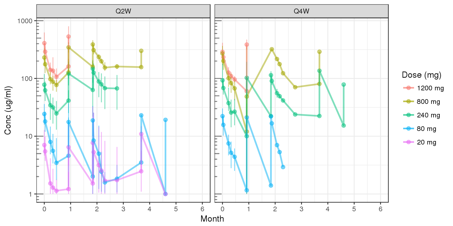

Concentration over time, faceted by regimen and cycle number, colored by dose

gg = gg
gg = gg %+% filter(d,CYCLE %in% c(1,3))
gg = gg + aes(x=TMTPT,y=CONC)
gg = gg + facet_grid(CYCLE~REG,labeller=label_both,switch="y")
gg = gg + scale_x_units(units.input = "h",units.output="d",t.end = 28,increment=7) 
gg = gg + ylab("Conc (ug/ml)")
gg = gg + ggtitle("PK by Cycle")
print(gg)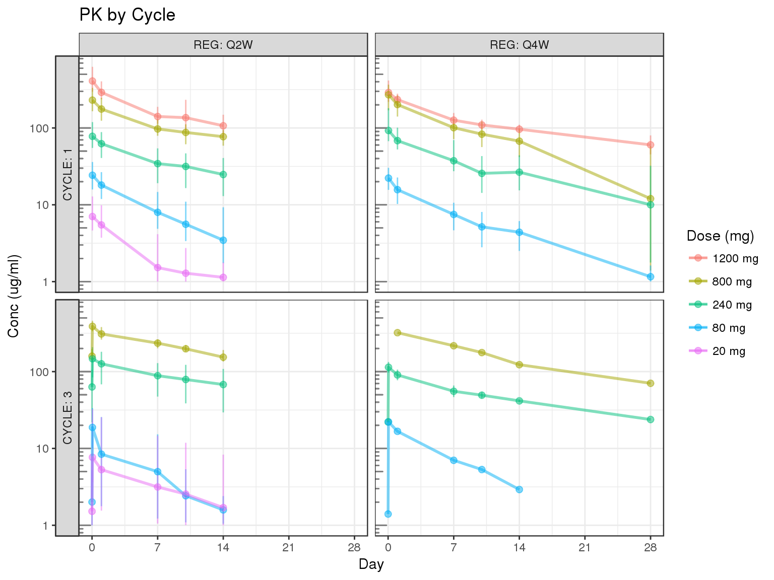

Assess the dose linearity of exposure

Dose normalized concentration

gg = ggplot(data = d, aes(x = NOMTIME, y = CONCnorm, color = DOSE0label, group=DOSE0label))
gg = gg + stat_summary(geom = "errorbar", width = 0.1, size = .5, 
                        fun.data = function(y){
                          y = stats::na.omit(y)
                          data.frame(
                          y = median(y),
                          ymin = quantile(y,.05),
                          ymax = quantile(y,.95)
                          )},alpha=.5) +  
  stat_summary(geom = "point", size = 2, fun.y = mean,alpha=.5) + 
  stat_summary(geom = "line", size = 1, fun.y = mean,alpha=.5) 
gg = gg + scale.y.log10()  + annotation_logticks(base = 10, sides = "l", color = rgb(0.5,0.5,0.5))
gg = gg + scale_x_units(units.input = "h",units.output="m",t.end = 6,increment=1) 
gg = gg + labs(color="Dose (mg)")
gg = gg + facet_grid(~REG)
gg = gg + ylab("Normalized Conc (ug/ml/mg)")
gg = gg + ggtitle("Normalized Concentration")
print(gg)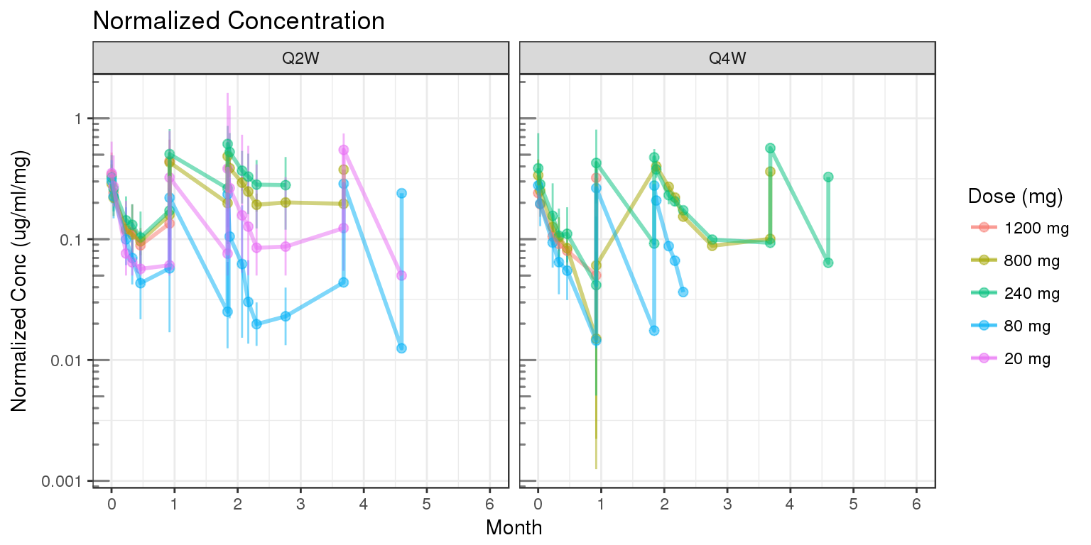

Noncompartmental Analysis

nca.filter = nca %>% 
  filter(WNLPARM %in% c("AUCINF_obs","AUClast","AUCtau","Cmax"))
g = ggplot(nca.filter,aes(x=DOSE0,y=PPORRESNnorm,group=DOSE0))
g = g + geom_boxplot(outlier.shape=NA)
g = g + geom_smooth(aes(group=NULL),show.legend = FALSE,se=FALSE)
g = g + geom_jitter(width=0,alpha=.3)
g = g + facet_grid(WNLPARM~REG,scales="free_y",switch="y")
g = g + scale.y.log10(.5)  + annotation_logticks(base = 10, sides = "l", color = rgb(0.5,0.5,0.5))
g = g + scale_x_log10(breaks=unique(d$DOSE0))
g = g + labs(x="First Dose (mg)",
             y="Normalized value (ug/ml/mg or ug/ml*d/mg)")
g = g + ggtitle("Normalized NCA")
print(g)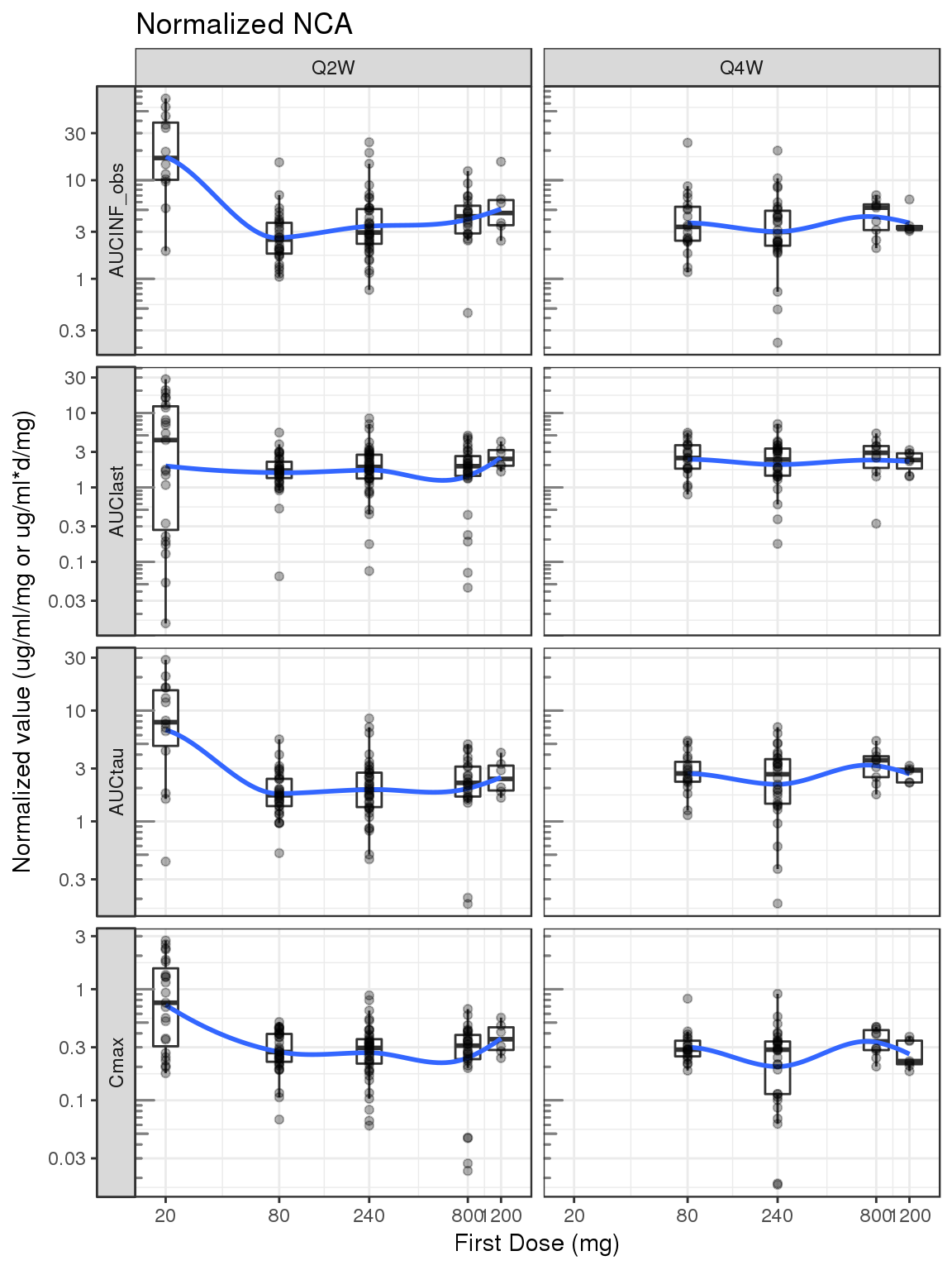

Explore variability

Spaghetti, grouped by dose

gg = ggplot(data = d, aes(x=TIME, y=CONC, group=ID))
gg = gg + geom_line(mapping=aes(group=ID),alpha = 0.5) 
gg = gg + geom_point(alpha = 0.5)
gg = gg + scale.y.log10()  + annotation_logticks(base = 10, sides = "l", color = rgb(0.5,0.5,0.5))
gg = gg + scale_x_units(units.input = "h",units.output="m",t.end = 6,increment=1) 
gg = gg + ylab("Conc (ug/ml)")
gg = gg + theme(legend.position="none")   
gg = gg + facet_grid(REG~DOSE0,switch="y")
print(gg)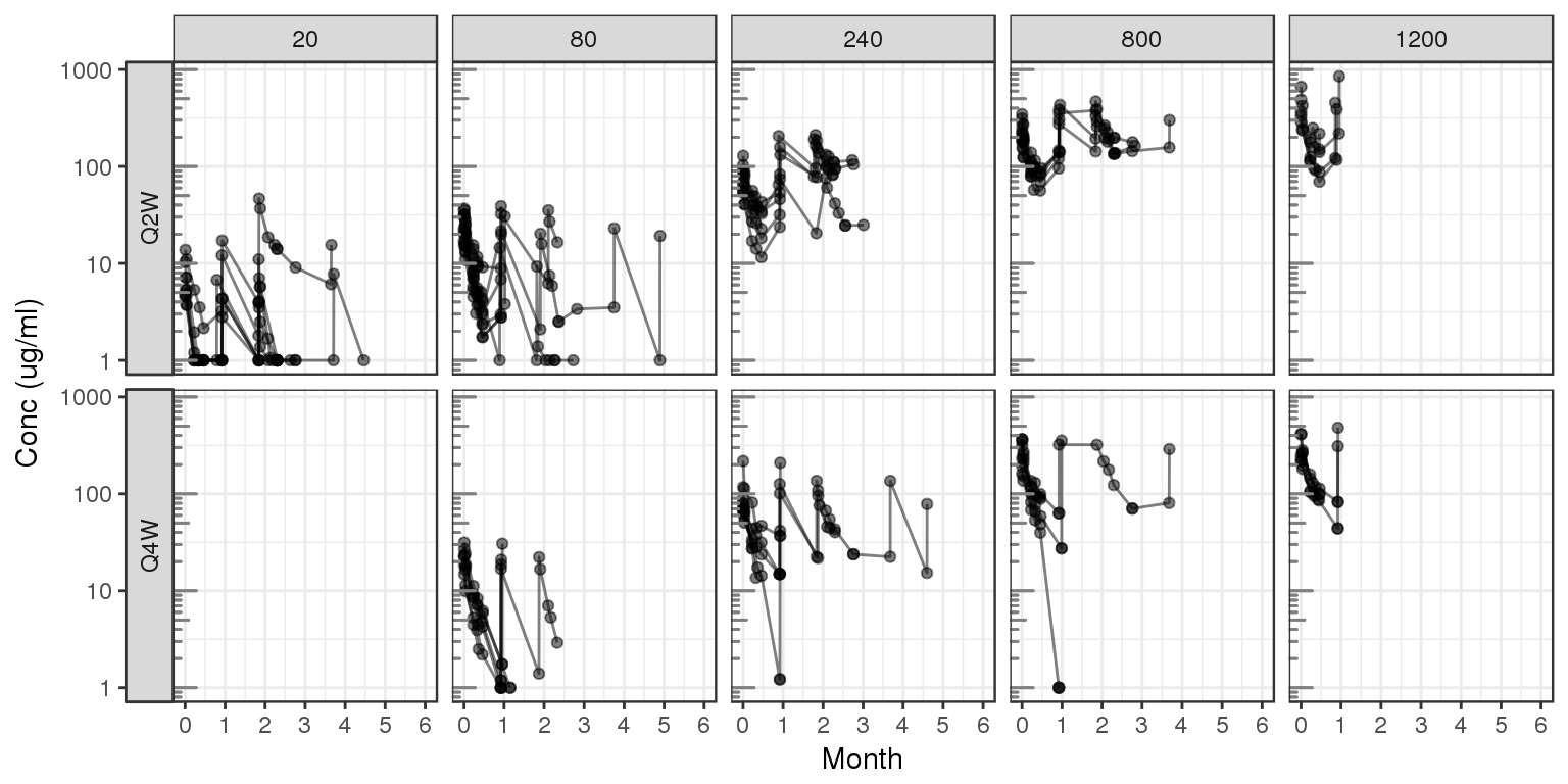

Explore irregularities in profiles

Individual profiles

gg = ggplot(data = d, aes(x=TIME, y=CONC, group=ID))
gg = gg + geom_line() 
gg = gg + geom_point()
gg = gg + scale.y.log10()  + annotation_logticks(base = 10, sides = "l", color = rgb(0.5,0.5,0.5))
gg = gg + scale_x_units(units.input = "h",units.output="m",t.end = 6,increment=1) 
gg = gg + ylab("Conc (ug/ml)")
gg = gg + theme(legend.position="none")   
gg = gg + facet_wrap(~DOSElabel+ID)
print(gg)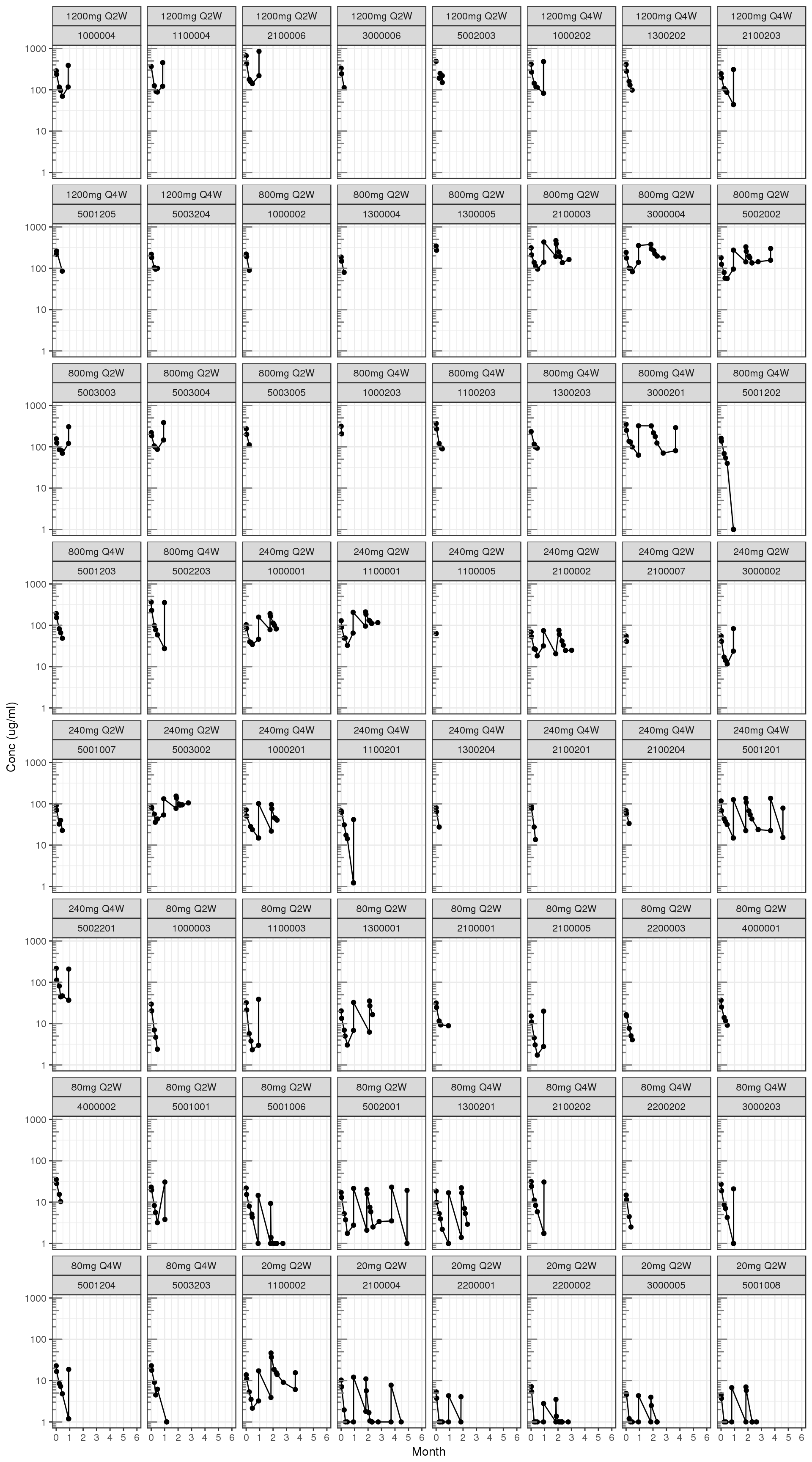

R Session Info

sessionInfo()

## R version 3.4.3 (2017-11-30)
## Platform: x86_64-pc-linux-gnu (64-bit)
## Running under: Red Hat Enterprise Linux Server 7.4 (Maipo)
## 
## Matrix products: default
## BLAS/LAPACK: /CHBS/apps/intel/17.4.196/compilers_and_libraries_2017.4.196/linux/mkl/lib/intel64_lin/libmkl_gf_lp64.so
## 
## locale:
##  [1] LC_CTYPE=en_US.UTF-8       LC_NUMERIC=C              
##  [3] LC_TIME=en_US.UTF-8        LC_COLLATE=en_US.UTF-8    
##  [5] LC_MONETARY=en_US.UTF-8    LC_MESSAGES=en_US.UTF-8   
##  [7] LC_PAPER=en_US.UTF-8       LC_NAME=C                 
##  [9] LC_ADDRESS=C               LC_TELEPHONE=C            
## [11] LC_MEASUREMENT=en_US.UTF-8 LC_IDENTIFICATION=C       
## 
## attached base packages:
## [1] grid      stats     graphics  grDevices utils     datasets  methods  
## [8] base     
## 
## other attached packages:
##  [1] lubridate_1.7.1 survival_2.41-3 DT_0.2          RxODE_0.6-1    
##  [5] bindrcpp_0.2    haven_1.1.0     readr_1.1.1     readxl_1.0.0   
##  [9] xtable_1.8-2    tidyr_0.7.2     caTools_1.17.1  zoo_1.8-0      
## [13] dplyr_0.7.4     ggplot2_2.2.1   gridExtra_2.3  
## 
## loaded via a namespace (and not attached):
##  [1] purrr_0.2.4        reshape2_1.4.3     splines_3.4.3     
##  [4] lattice_0.20-35    colorspace_1.3-2   htmltools_0.3.6   
##  [7] yaml_2.1.16        rlang_0.1.6        pillar_1.0.1      
## [10] glue_1.2.0         RColorBrewer_1.1-2 binom_1.1-1       
## [13] bindr_0.1          plyr_1.8.4         stringr_1.2.0     
## [16] munsell_0.4.3      gtable_0.2.0       cellranger_1.1.0  
## [19] htmlwidgets_0.9    codetools_0.2-15   evaluate_0.10.1   
## [22] memoise_1.1.0      labeling_0.3       knitr_1.18        
## [25] forcats_0.2.0      rex_1.1.2          markdown_0.8      
## [28] Rcpp_0.12.14       scales_0.5.0       backports_1.1.2   
## [31] jsonlite_1.5       hms_0.4.0          digest_0.6.13     
## [34] stringi_1.1.3      rprojroot_1.3-1    tools_3.4.3       
## [37] bitops_1.0-6       magrittr_1.5       lazyeval_0.2.1    
## [40] tibble_1.4.1       pkgconfig_2.0.1    Matrix_1.2-12     
## [43] rsconnect_0.8.5    assertthat_0.2.0   rmarkdown_1.8     
## [46] R6_2.2.2           compiler_3.4.3