PD, Dose-Response - Time to Event
Andy Stein, Anwesha Chaudhury, Alison Margolskee
Rmarkdown template to generate this page can be found on Rmarkdown-Template.
library(ggplot2)
library(dplyr)
library(broom)
library(knitr)
library(tidyr)
library(survival)
library(survminer)
library(xgxr)
set.seed(123456)
Explore Dose-Response Relationship
Create a Dataset
#Use the lung dataset to create a fake dose-response dataset
km_data <- lung %>%
  mutate(dose = ph.ecog) %>%
  filter(dose!=3) %>%
  mutate(dose_label = paste(dose," mg")) %>%
  select(time, dose, dose_label, status, sex)

#these columns are required for your dataset
km_data <- km_data %>%
  mutate(dose   = dose,   #dose,
         time   = time,   #time of the event (or censoring)
         event  = status) #status: there are a three options for this column (see ?Surv)
#        a) 0 = censored (alive), 1 = dead (event)
#        b) 1 = censored (alive), 2 = dead (event)
#        c) 0 = right censored, 1 = event at time,
#           2 = left censored,  3 = interval censored.
Plot Kaplan Meier with Confidence Intervals stratifying by dose
Time-to-event plots can be summarized by Kaplan-Meier plots and stratified by dose to give an overview of the dose-response. To see if there’s an effect on exposure vs response, look to see if there is separation between the doses.
km_fit <- survfit(Surv(time, status) ~ dose_label, data = km_data, conf.int = 0.95)
gg <- ggsurvplot(km_fit, km_data, conf.int = TRUE, ggtheme = xgx_theme())
gg <- gg + xgx_scale_x_time_units(units_dataset = "day", units_plot = "year")
print(gg)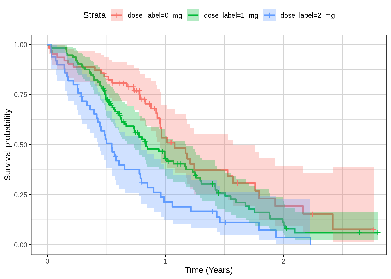
Plot Kaplan Meier faceted by exposure quartile for assessing covariates
This plot can help in assessing the impact of a covariate (sex) on outcome.
km_fit_sex <- survfit(Surv(time, status) ~ sex,
                       data = km_data,
                       conf.int = 0.95)
gg <- ggsurvplot_facet(km_fit_sex,
                       km_data,
                       facet.by = c("dose_label"),
                       conf.int = TRUE,
                       ggtheme = xgx_theme(),
                       legend.labs = paste0("SEX=",sort(unique(km_data$sex))))
gg <- gg + xgx_scale_x_time_units(units_dataset = "day", units_plot = "year")
print(gg)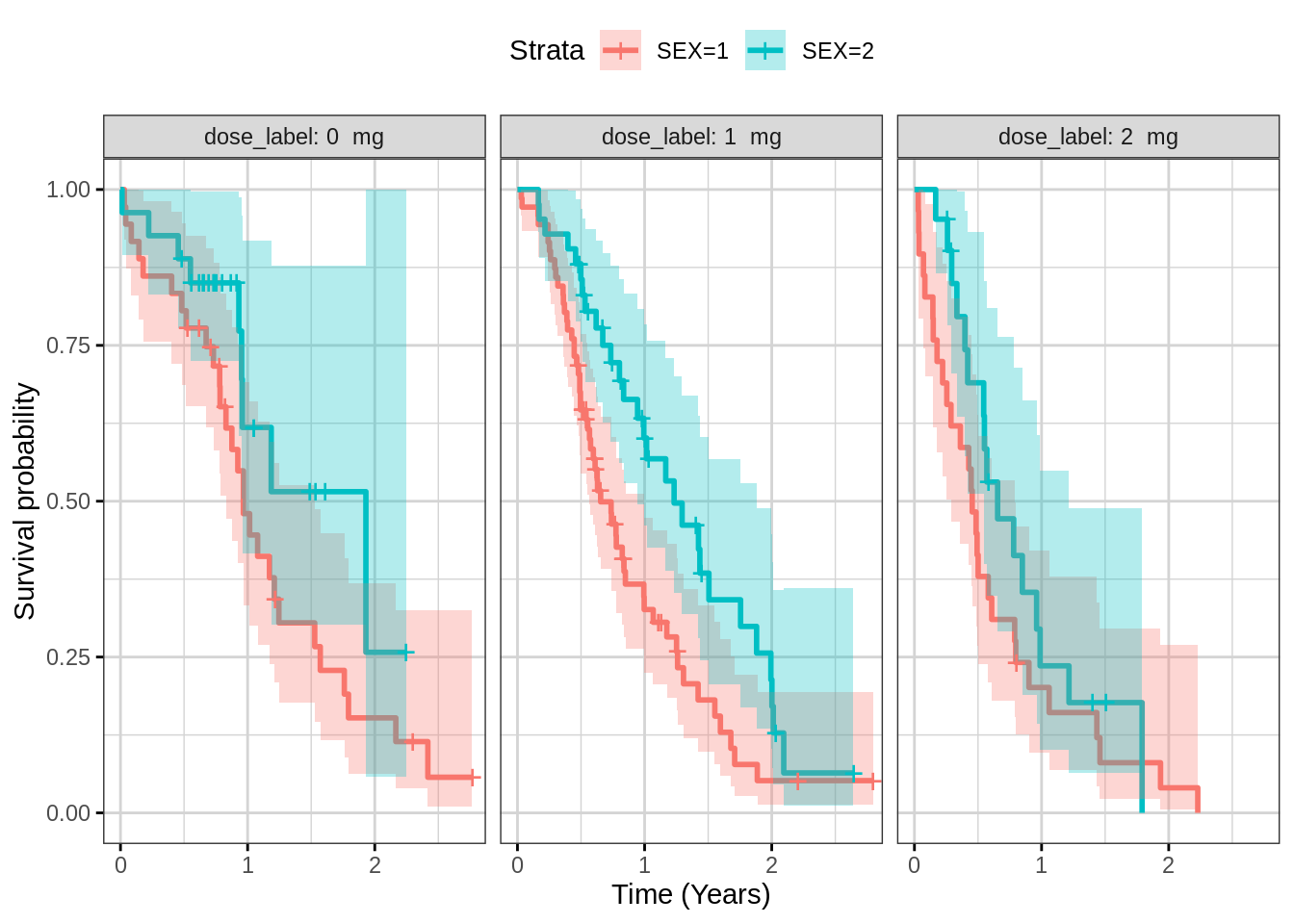
Performing Cox regression on the above data.
In this data only a few variables are available, so variable selection isn’t needed. If there are multiple variables, applying a variable selection approach (e.g. stepwiseAIC) would be advisable. Look for small p values or large hazard ratios to identify covariates that have a large effect.
km_cox <- coxph(Surv(time) ~ dose + sex,
             data =km_data)
km_cox_summary <- broom::tidy(km_cox) %>%
  mutate_at(vars(-term),signif,2)
kable(km_cox_summary) | term | estimate | std.error | statistic | p.value |
|---|---|---|---|---|
| dose | 0.29 | 0.098 | 2.9 | 0.0033 |
| sex | -0.21 | 0.140 | -1.5 | 0.1300 |
Mean Event Rate over time
For repeated time to event data, the rate of occurance of the events can be plotted. The observed average rate of occurance would be related to the Hazard rate in a time-to-event model.
Calculate the rate of occurance of an event as the number of events occuring within specific time intervals, average over the number of subjects being observed.
Observe the mean event rate, do you see any patterns? Does the event rate increase or decrease over time, or at specific time points (e.g. dosing intervals, circadian rhythms)?
# (coming soon)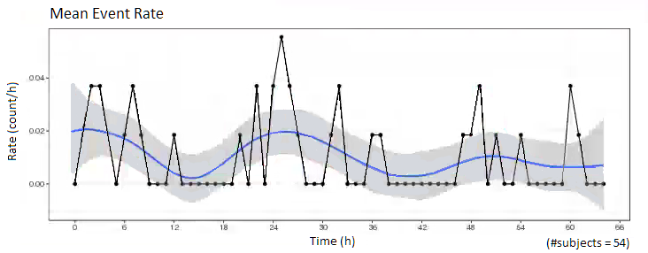
Mean Cumulative Function
The mean cumulative function is another way of looking at repeated time-to-event data. The mean cumulative function is the population average of the cumulative number of events over time, and would be related to the Cumulative Hazard in a time-to-event model.
Calculate the mean cumulative function by ordering all of the events by increasing time, calculate the cumulative number of occurances up to each time point, and take the average over the number of subjects being observed. For repeated time-to-event data, the mean cumulative function can achieve values greater than 1.
# (coming soon)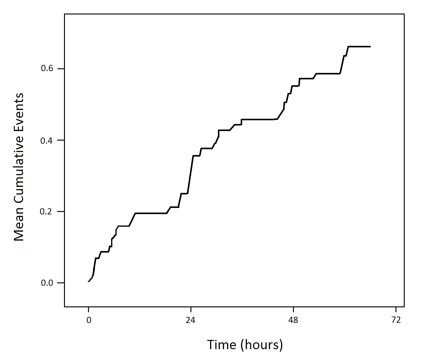
R Session Info
sessionInfo()## R version 4.1.0 (2021-05-18)
## Platform: x86_64-pc-linux-gnu (64-bit)
## Running under: Red Hat Enterprise Linux Server 7.9 (Maipo)
##
## Matrix products: default
## BLAS/LAPACK: /CHBS/apps/EB/software/imkl/2019.1.144-gompi-2019a/compilers_and_libraries_2019.1.144/linux/mkl/lib/intel64_lin/libmkl_gf_lp64.so
##
## locale:
## [1] LC_CTYPE=en_US.UTF-8 LC_NUMERIC=C LC_TIME=en_US.UTF-8 LC_COLLATE=en_US.UTF-8 LC_MONETARY=en_US.UTF-8
## [6] LC_MESSAGES=en_US.UTF-8 LC_PAPER=en_US.UTF-8 LC_NAME=C LC_ADDRESS=C LC_TELEPHONE=C
## [11] LC_MEASUREMENT=en_US.UTF-8 LC_IDENTIFICATION=C
##
## attached base packages:
## [1] stats graphics grDevices utils datasets methods base
##
## other attached packages:
## [1] survminer_0.4.9 ggpubr_0.4.0 survival_3.4-0 knitr_1.40 broom_1.0.1 caTools_1.18.2 DT_0.26 forcats_0.5.2 stringr_1.4.1
## [10] purrr_0.3.5 readr_2.1.3 tibble_3.1.8 tidyverse_1.3.2 xgxr_1.1.1 zoo_1.8-11 gridExtra_2.3 tidyr_1.2.1 dplyr_1.0.10
## [19] ggplot2_3.3.6
##
## loaded via a namespace (and not attached):
## [1] googledrive_2.0.0 colorspace_2.0-3 ggsignif_0.6.2 deldir_1.0-6 rio_0.5.27 ellipsis_0.3.2 class_7.3-19
## [8] htmlTable_2.2.1 markdown_1.2 base64enc_0.1-3 fs_1.5.2 gld_2.6.2 rstudioapi_0.14 proxy_0.4-26
## [15] farver_2.1.1 Deriv_4.1.3 fansi_1.0.3 mvtnorm_1.1-3 lubridate_1.8.0 xml2_1.3.3 codetools_0.2-18
## [22] splines_4.1.0 cachem_1.0.6 rootSolve_1.8.2.2 Formula_1.2-4 jsonlite_1.8.3 km.ci_0.5-2 binom_1.1-1
## [29] cluster_2.1.3 dbplyr_2.2.1 png_0.1-7 compiler_4.1.0 httr_1.4.4 backports_1.4.1 assertthat_0.2.1
## [36] Matrix_1.5-1 fastmap_1.1.0 gargle_1.2.1 cli_3.4.1 prettyunits_1.1.1 htmltools_0.5.3 tools_4.1.0
## [43] gtable_0.3.1 glue_1.6.2 lmom_2.8 Rcpp_1.0.9 carData_3.0-4 cellranger_1.1.0 jquerylib_0.1.4
## [50] vctrs_0.5.0 nlme_3.1-160 crosstalk_1.2.0 xfun_0.34 openxlsx_4.2.4 rvest_1.0.3 lifecycle_1.0.3
## [57] rstatix_0.7.0 googlesheets4_1.0.1 MASS_7.3-58.1 scales_1.2.1 hms_1.1.2 expm_0.999-6 RColorBrewer_1.1-3
## [64] curl_4.3.3 yaml_2.3.6 Exact_2.1 KMsurv_0.1-5 pander_0.6.4 sass_0.4.2 rpart_4.1.16
## [71] reshape_0.8.8 latticeExtra_0.6-30 stringi_1.7.8 highr_0.9 e1071_1.7-8 checkmate_2.1.0 zip_2.2.0
## [78] boot_1.3-28 rlang_1.0.6 pkgconfig_2.0.3 bitops_1.0-7 evaluate_0.17 lattice_0.20-45 htmlwidgets_1.5.4
## [85] labeling_0.4.2 tidyselect_1.2.0 GGally_2.1.2 plyr_1.8.7 magrittr_2.0.3 R6_2.5.1 DescTools_0.99.42
## [92] generics_0.1.3 Hmisc_4.7-0 DBI_1.1.3 pillar_1.8.1 haven_2.5.1 foreign_0.8-82 withr_2.5.0
## [99] mgcv_1.8-41 abind_1.4-5 RCurl_1.98-1.4 nnet_7.3-17 car_3.0-11 crayon_1.5.2 modelr_0.1.9
## [106] survMisc_0.5.5 interp_1.1-2 utf8_1.2.2 tzdb_0.3.0 rmarkdown_2.17 progress_1.2.2 jpeg_0.1-9
## [113] grid_4.1.0 readxl_1.4.1 minpack.lm_1.2-1 data.table_1.14.2 reprex_2.0.2 digest_0.6.30 xtable_1.8-4
## [120] munsell_0.5.0 bslib_0.4.0