Data Checking

Overview

This file runs initial data analysis (IDA) on a modeling dataset, before any modeling begins. The aim of IDA is to confirm that the data match your expectations and are ready for analysis, without touching the research question itself (Baillie et al. 2022, Ten Simple Rules for IDA).

For a dataset that is much larger that the example one used here, the default figure size may be too small for all plots to be readable. In that case, add or edit the fig.height and fig.width in the top of each chunk. For example: {r, fig.height = 6, fig.width = 8}

Data specifications can be accessed on Datasets and Rmarkdown template to generate this page can be found on Rmarkdown-Template. You may also download the Multiple Ascending Dose PK/PD dataset for your reference (download dataset).

What this document covers

This document uses the STRATOS framework developed by an international initiative for STRengthening Analytical Thinking for Observational Studies. It roughly follows the first three phases of that framework (metadata, data cleaning, data screening), with the sections below organized around the concrete questions a modeler asks.

#	Section	Question it answers
1	About This Data	What is this dataset — where did it come from?
2	Subject and Record Accounting	Do the subject and record counts, by study and treatment arm, match expectations?
3	Checking Values Are Valid	Are the dose, observation, and timing values legitimate and internally consistent? Includes plotting the data, cross-column integrity checks, and BLQ.
4	Missing Data	How much is missing, what is missing together, and does missingness relate to other variables?
5	Distributions and Relationships	How are the covariates and observations distributed, and which are correlated?
6	Summary of Findings	What did the checks reveal that a modeler should keep in mind?

The document ends by providing the modeler with a list of considerations around what further issues with the data should be addressed and how the analysis plan might change based on the IDA.

Setup

library(tidyverse)
library(xgxr)
library(DT)
library(GGally)

xgx_theme_set()
filter <- dplyr::filter #have filter be dplyr::filter instead of stats::filter

status <- "DRAFT"

#caption
Rmd_name <- "Data_Checking.Rmd"
parent_dir <- "/top/level/directory/"
project_dir <- "./"

caption <- paste(
  c(
    paste0(parent_dir, project_dir, "/pgm"),
    Rmd_name,
    str_replace(Rmd_name, "\\.Rmd$", ".html"),
    format(Sys.time(), "%Y-%m-%d %H:%M")
  ),
  collapse = "\n"
)

ggcaption <- list(
  labs(caption = caption),
  theme(plot.caption = element_text(hjust = 0.5))
)

# chunk defaults
knitr::opts_chunk$set(
  warning = FALSE,
  message = FALSE,
  fig.height = 4,
  fig.width = 4
)
options(DT.options = list(pageLength = 20))

# --- Analysis-specific settings: EDIT THESE for your dataset -----------------

# Path to the modeling dataset to check, relative to this .Rmd. The site build
# renders from inside Rmarkdown/, which is why this is "../Data/..." and not
# "Data/..." -- the same convention every other page here uses. A bare
# "Data/..." works when you run chunks interactively from the project root and
# then fails in the build.
filename <- "../Data/Data_Checking.csv"
modeling_data_in <- read.csv(filename, stringsAsFactors = FALSE)

# time units of the dataset (used for axis scaling)
time_units_dataset <- "days"

# covariates to summarize in the IDA section
covariates <- c("AGE0", "WEIGHT0", "SEX")

# --- Metadata: plausibility ranges for continuous variables ------------------
# Used by the "Plausibility Range Checks" section. Add one row per continuous
# variable you want range-checked. Values outside [lower, upper] are flagged.
# EDIT THIS for your dataset.
plausibility_ranges <- tibble::tribble(
  ~variable , ~lower , ~upper ,
  "AGE0"    ,     18 ,     90 ,
  "WEIGHT0" ,     30 ,    200 ,
)

# --- Metadata: expected categorical values -----------------------------------
# Used by the "Plausibility Range Checks" section. Any observed level not in the
# allowed set is flagged. EDIT THIS for your dataset (or leave empty to skip).

allowed_levels <- list(
  CENS = c(0, 1),
  EVID = c(0, 1),
  MDV = c(0, 1)
)

# --- Metadata: assay and dosing conventions ----------------------------------
# EDIT THESE for your dataset.

# Column holding the lower limit of quantification, or NA if the dataset does
# not carry one. Used by the BLQ section to check CENS against the LLOQ.
lloq_col <- "LLOQ"

# Covariates that must not change within a subject. The document summarizes
# covariates from the first record per subject, which is only valid if this
# holds -- so it is checked rather than assumed.
subject_invariant <- c("AGE0", "WEIGHT0", "SEX", "AGEB", "WEIGHTB", "TRT")

# Value of NAME that marks a dosing record, used for time-after-dose.
name_dose <- "Dose"

Load Data

The mutate() below maps your dataset’s columns onto the standard names used throughout this document. If your dataset uses a different naming convention, edit the right-hand side of each assignment.

data_in <- modeling_data_in

data <- data_in %>%
  mutate(
    STUDYID = STUDYID, # Study identifier
    USUBJID = USUBJID, # Unique subject identifier
    TIME = TIME, # Actual time
    NOMTIME = NOMTIME, # Nominal time
    AMT = AMT, # Dose amount
    LIDV = LIDV, # Dependent variable
    YTYPE = YTYPE, # Number for type of dependent variable
    NAME = NAME, # Name for the type of dependent variable (e.g. PK)
    MDV = MDV, # Missing dependent variable (0 = no, 1 = yes)
    CENS = CENS, # Censored data (0 = no, 1 = yes)
    EVID = EVID, # Event ID. 0 = observation, 1 = dose
    TRT = TRT, # Treatment arm character description
    TRTN = TRTN
  ) %>% # Treatment arm numeric description (for sorting)
  arrange(TRTN) %>%
  mutate(
    TRT_low2high = factor(TRT, levels = unique(TRT)),
    TRT_high2low = factor(TRT, levels = rev(unique(TRT)))
  )

# one row per subject, for covariate summaries
data1 <- data %>%
  filter(!duplicated(USUBJID))

Covariates are read from the first record per subject (data1), which is only valid if they genuinely do not change within a subject. That is a strong assumption and a quiet one — if it fails, every covariate summary, distribution and correlation below is computed from an arbitrary first row and still looks perfectly clean. So it is checked, not assumed: see Dataset Integrity Checks, which lists any variable in subject_invariant that moves within a subject.

About this dataset

Record where the data came from and what it should contain, so the analysis is reproducible and its expectations are explicit. Anyone re-running this file should be able to see exactly which file was checked and when.

provenance <- tibble::tibble(
  item = c(
    "Source file",
    "File last modified",
    "Report run at",
    "N rows",
    "N columns",
    "N subjects (USUBJID)",
    "N treatment arms"
  ),
  value = c(
    normalizePath(filename, mustWork = FALSE),
    as.character(file.info(filename)$mtime),
    format(Sys.time(), "%Y-%m-%d %H:%M"),
    format(nrow(data), big.mark = ","),
    as.character(ncol(data)),
    as.character(dplyr::n_distinct(data$USUBJID)),
    as.character(dplyr::n_distinct(data$TRT))
  )
)
datatable(provenance, options = list(dom = "t"))

Subject and Record Accounting

Confirm that the number of subjects and records — overall and broken out by study and treatment arm — matches expectations.

Subject Accountability

Account for how many subjects survive each selection step, from the raw file to the analysis-ready dataset. Edit the steps to match the filters your dataset actually applies. Unexpected drops here are often the first sign of a data problem.

n_subj <- function(df) dplyr::n_distinct(df$USUBJID)

# EDIT THESE steps to reflect the selection applied to your dataset.
accountability <- tibble::tibble(
  step = c(
    "Subjects in source file",
    "With at least one dose record (EVID == 1)",
    "With at least one observation (EVID == 0)",
    "With non-missing treatment arm (TRT)"
  ),
  n_subjects = c(
    n_subj(data_in %>% mutate(USUBJID = USUBJID)),
    n_subj(data %>% filter(EVID == 1)),
    n_subj(data %>% filter(EVID == 0)),
    n_subj(data %>% filter(!is.na(TRT)))
  )
) %>%
  mutate(dropped_from_previous = dplyr::lag(n_subjects) - n_subjects)

datatable(accountability, options = list(dom = "t"))

Number of Patients per Treatment Arm

Check that the number of patients in the dataset is what you expect.

total_patients <- data %>%
  filter(!duplicated(USUBJID)) %>%
  group_by(STUDYID) %>%
  tally() %>%
  rename(n_patients = n) %>%
  mutate(TRT_low2high = "TOTAL NUMBER")

summary_by_trt <- data %>%
  filter(!duplicated(USUBJID)) %>%
  group_by(STUDYID, TRT_low2high) %>%
  tally() %>%
  rename(n_patients = n) %>%
  bind_rows(total_patients) %>%
  arrange(STUDYID, TRT_low2high)

datatable(summary_by_trt)

Number of Data Points per Treatment Arm and YTYPE

Another quick way to see if there is more or less data than expected.

summary_by_trt_ytype <- data %>%
  group_by(STUDYID, YTYPE, NAME, TRT_low2high) %>%
  tally() %>%
  rename(n_data_points = n) %>%
  mutate(YTYPE_NAME = paste0(YTYPE, ":", NAME)) %>%
  ungroup() %>%
  select(-YTYPE, -NAME) %>%
  spread(YTYPE_NAME, n_data_points) %>%
  arrange(STUDYID, TRT_low2high)

datatable(summary_by_trt_ytype)

Checking Values Are Valid

Confirm that the dose, observation, and timing values are legitimate and internally consistent — no impossible values, unexpected zeros, or mismatched times.

Dosing Summary

It can be useful to know if there are patients who never received a dose, and AMT usually should not equal 0.

dose <- data %>%
  filter(EVID == 1)

dose_summ <- data %>%
  group_by(USUBJID) %>%
  summarize(total_dose = sum(AMT))

dose_summary <- data.frame(
  patients_that_never_received_drug = sum(dose_summ$total_dose == 0),
  entries_where_AMT_equals_0 = sum(dose$AMT == 0),
  entries_where_AMT_greater_than_0 = sum(dose$AMT > 0)
) %>%
  t() %>%
  as.data.frame() %>%
  rename(N = V1)

datatable(dose_summary)

Dependent Variable (DV) Summary

# number of DV by YTYPE and by patient (NAs count as 0)
# keep EVID == 1 records so patients with a dose but no DV are still counted
dv_number_by_patient <- data %>%
  group_by(YTYPE, USUBJID) %>%
  summarize(n_obs = sum(MDV == 0 & !is.na(LIDV))) %>%
  ungroup() %>%
  spread(YTYPE, n_obs)

dv_number_summary <- dv_number_by_patient %>%
  select(-USUBJID) %>%
  summarize_all(c(
    Nnone = function(x) sum(x == 0 | is.na(x)),
    Nmin = function(x) min(x, na.rm = TRUE),
    Nmedian = function(x) round(median(x, na.rm = TRUE)),
    Nmax = function(x) max(x, na.rm = TRUE)
  )) %>%
  t() %>%
  as.data.frame() %>%
  rename(N = V1)
dv_number_summary$YTYPE_SUMM <- row.names(dv_number_summary)
dv_number_summary <- dv_number_summary %>%
  mutate(
    YTYPE = as.numeric(str_extract(YTYPE_SUMM, "^\\d+")),
    SUMM = str_extract(YTYPE_SUMM, "[A-Za-z]+$")
  ) %>%
  select(-YTYPE_SUMM) %>%
  spread(SUMM, N)

dv_summary_overall <- data %>%
  filter(EVID == 0) %>%
  group_by(YTYPE, NAME) %>%
  summarize(
    n_total = n(),
    n_missing_or_NA = sum(is.na(LIDV) | MDV == 1),
    # na.rm throughout: without it a single NA observation turns the whole
    # count into NA and the column silently goes blank.
    n_zeroes = sum(LIDV == 0, na.rm = TRUE),
    n_censored = sum(CENS == 1, na.rm = TRUE),
    n_negative = sum(LIDV < 0, na.rm = TRUE),
    n_duplicate_times = sum(duplicated(paste(USUBJID, TIME))),
    min = min(LIDV, na.rm = TRUE),
    Q1 = quantile(LIDV, 0.25, na.rm = TRUE),
    median = median(LIDV, na.rm = TRUE),
    Q3 = quantile(LIDV, 0.75, na.rm = TRUE),
    max = max(LIDV, na.rm = TRUE)
  ) %>%
  # round DV summary stats to 3 significant digits (any magnitude, no forced
  # scientific notation); counts are already integers and left alone
  mutate(across(c(min, Q1, median, Q3, max), ~ signif(.x, 3))) %>%
  left_join(dv_number_summary, by = "YTYPE") %>%
  mutate(YTYPE_NAME = paste0(YTYPE, ":", NAME)) %>%
  ungroup() %>%
  select(-YTYPE, -NAME) %>%
  t() %>%
  as.data.frame()
names(dv_summary_overall) <- as.matrix(dv_summary_overall["YTYPE_NAME", ])
dv_summary_overall$Value <- row.names(dv_summary_overall)
row.names(dv_summary_overall) <- c()

dv_summary_overall <- dv_summary_overall %>%
  filter(Value != "YTYPE_NAME") %>%
  mutate(
    Type = case_when(
      str_detect(Value, "^n_") ~ "Number of data points",
      str_detect(Value, "^N") ~ "Number of data points per patient",
      TRUE ~ "Value of data points"
    )
  ) %>%
  mutate(
    Value = str_replace(Value, "^n_", ""),
    Value = str_replace(Value, "^N", "")
  ) %>%
  select(Type, Value, everything()) %>%
  arrange(Type)

datatable(dv_summary_overall)

Look at the Data

Before any summary statistic, plot the dependent variable against time. Most data errors that matter are visible here and nowhere else: a profile with the wrong units, a subject whose doses were never recorded, a decimal-point slip, a concentration that rises when it should fall.

Linear and semi-log side by side, because they fail differently — the linear panel shows the peak, the log panel shows the terminal phase and anything impossibly low.

obs <- data %>% filter(EVID == 0)

gg <- ggplot(obs, aes(x = TIME, y = LIDV, group = USUBJID, color = TRT_low2high)) +
  geom_line(alpha = 0.5) +
  geom_point(size = 0.8, alpha = 0.7) +
  facet_wrap(~NAME, scales = "free_y") +
  xgx_scale_x_time_units(units_dataset = time_units_dataset) +
  labs(y = "Observed value", color = "Treatment") +
  xgx_annotate_status(status)

print(gg)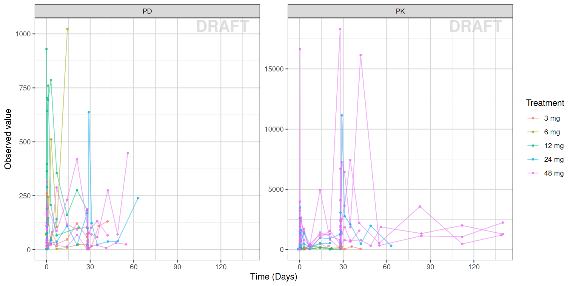

print(gg + xgx_scale_y_log10() + labs(y = "Observed value (log scale)"))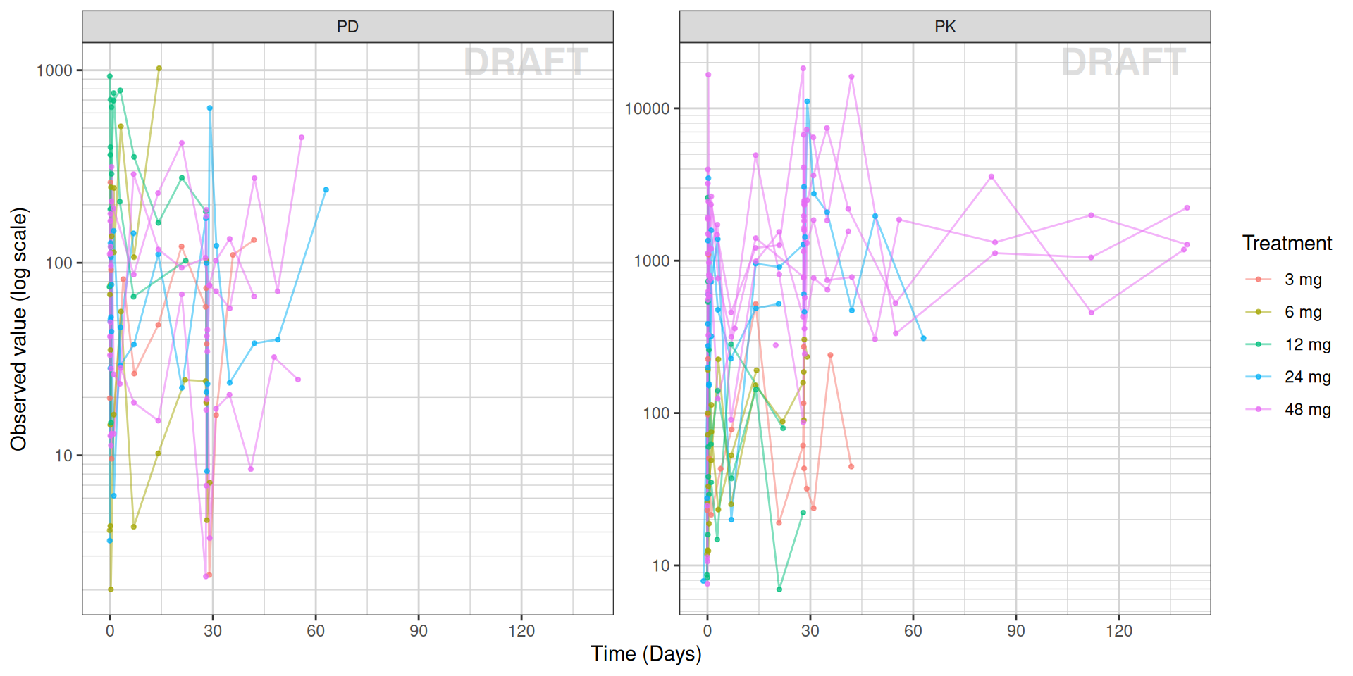

Time After Dose

Overlaying profiles on time-after-dose collapses the dosing schedule and makes the shape of a single interval visible. It is also a check in its own right: every observation should have a dose before it, and TAD should never be negative. Observations with no preceding dose show up as NA and are counted below.

# Running maximum of dosing times gives the most recent dose at each row in a
# single pass, without a many-to-many join that would blow up on a large study.
data_tad <- data %>%
  arrange(USUBJID, TIME) %>%
  group_by(USUBJID) %>%
  mutate(last_dose_time = cummax(ifelse(EVID == 1, TIME, -Inf))) %>%
  ungroup() %>%
  mutate(
    last_dose_time = ifelse(is.infinite(last_dose_time), NA, last_dose_time),
    TAD = TIME - last_dose_time
  )

n_no_prior_dose <- sum(data_tad$EVID == 0 & is.na(data_tad$TAD))
cat("Observations with no preceding dose record:", n_no_prior_dose, "\n")

## Observations with no preceding dose record: 20

gg_tad <- data_tad %>%
  filter(EVID == 0, !is.na(TAD)) %>%
  ggplot(aes(x = TAD, y = LIDV, group = USUBJID, color = TRT_low2high)) +
  geom_line(alpha = 0.5) +
  geom_point(size = 0.8, alpha = 0.7) +
  facet_wrap(~NAME, scales = "free_y") +
  xgx_scale_x_time_units(units_dataset = time_units_dataset) +
  xgx_scale_y_log10() +
  labs(x = "Time after dose", y = "Observed value", color = "Treatment") +
  xgx_annotate_status(status)

print(gg_tad)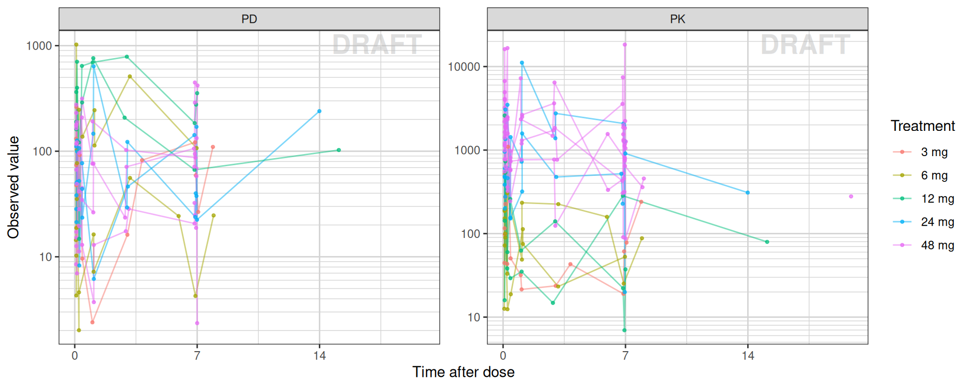

Plausibility Range Checks

Beyond min/max, check values against the ranges you declared in the setup chunk (plausibility_ranges and allowed_levels): a value can be non-missing and still be impossible. Empty tables mean no violations were found.

continuous_violations <- plausibility_ranges %>%
  filter(variable %in% names(data)) %>%
  mutate(
    n_violations = purrr::pmap_int(
      list(variable, lower, upper),
      function(variable_name, lo, hi) {
        x <- data[[variable_name]]

        sum(
          !is.na(x) & (x < lo | x > hi)
        )
      }
    )
  )

datatable(
  continuous_violations %>% filter(n_violations > 0),
  options = list(dom = "t"),
  caption = "Continuous variables with out-of-range values"
)

cat_violations <- purrr::imap_dfr(allowed_levels, function(allowed, var) {
  if (!var %in% names(data)) {
    return(NULL)
  }
  observed <- data[[var]]
  bad <- setdiff(unique(observed[!is.na(observed)]), allowed)
  if (length(bad) == 0) {
    return(NULL)
  }
  tibble::tibble(
    variable = var,
    allowed = paste(allowed, collapse = ", "),
    unexpected_values = paste(bad, collapse = ", "),
    n_rows = sum(observed %in% bad)
  )
})

if (nrow(cat_violations) == 0) {
  cat("No unexpected categorical values found.\n")
} else {
  datatable(
    cat_violations,
    options = list(dom = "t"),
    caption = "Categorical variables with unexpected values"
  )
}

## No unexpected categorical values found.

Dataset Integrity Checks

The plausibility checks above ask whether each value is individually legal. These ask whether the columns agree with each other, which is where most modelling-dataset defects actually live. A dataset can have a perfectly legal EVID, a perfectly legal AMT, and still be broken because a dosing record carries no dose.

The checks follow the conventions NONMEM enforces, and are modelled on the set in NMdata::NMcheckData() (Delff). Each is skipped automatically if the columns it needs are absent, so the block is safe to keep when your dataset has no CMT, ADDL or RATE.

has <- function(...) all(c(...) %in% names(data))
results <- list()
record <- function(check, n, note = "") {
  results[[length(results) + 1]] <<- tibble::tibble(
    check = check, n_failing = as.integer(n), note = note
  )
}

# --- timing ------------------------------------------------------------------
if (has("USUBJID", "TIME")) {
  dec <- data %>%
    group_by(USUBJID) %>%
    mutate(decreasing = TIME < lag(TIME)) %>%
    ungroup()
  record(
    "TIME decreases within a subject", sum(dec$decreasing, na.rm = TRUE),
    "NONMEM requires non-decreasing TIME within an individual"
  )
}

# --- duplicate events --------------------------------------------------------
dup_key <- intersect(c("USUBJID", "CMT", "EVID", "TIME"), names(data))
dup_rows <- data[duplicated(data[, dup_key]), , drop = FALSE]
record(
  paste0("Duplicate events on ", paste(dup_key, collapse = " + ")),
  nrow(dup_rows), "Exact repeats of the same event key"
)

# --- EVID / AMT / MDV / DV agreement -----------------------------------------
if (has("EVID", "AMT")) {
  record("Dosing record (EVID==1) with AMT missing or <= 0",
         sum(data$EVID == 1 & (is.na(data$AMT) | data$AMT <= 0)))
  record("Observation record (EVID==0) with AMT > 0",
         sum(data$EVID == 0 & !is.na(data$AMT) & data$AMT > 0))
}
if (has("EVID", "MDV", "LIDV")) {
  record("MDV==0 but the dependent variable is missing",
         sum(data$EVID == 0 & data$MDV == 0 & is.na(data$LIDV)))
  record("MDV==1 but a dependent variable is present",
         sum(data$EVID == 0 & data$MDV == 1 & !is.na(data$LIDV)))
}

# --- compartment -------------------------------------------------------------
if (has("CMT")) {
  record("CMT not a positive integer",
         sum(is.na(data$CMT) | data$CMT <= 0 | data$CMT != round(data$CMT)))
  if (has("YTYPE")) {
    multi <- data %>%
      filter(EVID == 0) %>%
      distinct(YTYPE, CMT) %>%
      count(YTYPE) %>%
      filter(n > 1)
    record("YTYPE mapping to more than one CMT", nrow(multi))
  }
}

# --- subject completeness ----------------------------------------------------
if (has("USUBJID", "EVID")) {
  per_subj <- data %>%
    group_by(USUBJID) %>%
    summarise(doses = sum(EVID == 1), obs = sum(EVID == 0), .groups = "drop")
  record("Subjects with no dosing record", sum(per_subj$doses == 0))
  record("Subjects with no observation record", sum(per_subj$obs == 0))
}
if (has("ID", "USUBJID")) {
  record("ID and USUBJID not one-to-one",
         abs(nrow(distinct(data, ID, USUBJID)) - n_distinct(data$USUBJID)))
}

# --- covariates that must not move within a subject --------------------------
inv <- intersect(subject_invariant, names(data))
inv_varying <- tibble::tibble(variable = character(), n_subjects = integer())
if (length(inv) > 0) {
  inv_varying <- data %>%
    group_by(USUBJID) %>%
    summarise(across(all_of(inv), ~ n_distinct(.x[!is.na(.x)]) > 1), .groups = "drop") %>%
    select(all_of(inv)) %>%
    summarise(across(everything(), ~ sum(.x))) %>%
    pivot_longer(everything(), names_to = "variable", values_to = "n_subjects") %>%
    filter(n_subjects > 0)
  record("Subject-invariant covariates that vary within a subject",
         nrow(inv_varying),
         "Covariate summaries take the first record per subject, so this must be zero")
}

# --- units -------------------------------------------------------------------
unit_cols <- intersect(c("UNIT", "EVENTU"), names(data))
if (length(unit_cols) > 0 && has("NAME")) {
  mixed <- data %>%
    filter(EVID == 0) %>%
    group_by(NAME) %>%
    summarise(across(all_of(unit_cols), ~ n_distinct(.x)), .groups = "drop") %>%
    pivot_longer(-NAME) %>%
    filter(value > 1)
  record("Analytes carrying more than one unit", nrow(mixed))
}

# --- optional NONMEM columns, only if present --------------------------------
if (has("RATE")) {
  record("RATE neither -2, -1 nor non-negative",
         sum(!is.na(data$RATE) & data$RATE < 0 & !data$RATE %in% c(-1, -2)))
}
if (has("SS")) {
  record("SS not 0 or 1", sum(!is.na(data$SS) & !data$SS %in% c(0, 1)))
}
if (has("ADDL", "II")) {
  record("ADDL present without a positive II",
         sum(!is.na(data$ADDL) & data$ADDL > 0 & (is.na(data$II) | data$II <= 0)))
}

integrity <- bind_rows(results) %>%
  mutate(status = ifelse(n_failing == 0, "pass", "REVIEW")) %>%
  select(status, check, n_failing, note) %>%
  arrange(status, desc(n_failing))

datatable(integrity, options = list(pageLength = 25, dom = "t"),
          caption = "Dataset integrity checks")

Anything marked REVIEW is detailed below.

if (nrow(inv_varying) > 0) {
  datatable(
    inv_varying,
    options = list(dom = "t"),
    caption = "Covariates that change within a subject (should be none)"
  )
} else {
  cat("All subject-invariant covariates are constant within subject.\n")
}

if (nrow(dup_rows) > 0) {
  datatable(
    dup_rows %>% select(any_of(c("USUBJID", "TIME", "EVID", "CMT", "NAME", "LIDV"))),
    caption = "Duplicated event records"
  )
} else {
  cat("No duplicated event records.\n")
}

Below the Limit of Quantification (BLQ)

How much of the data is below the assay limit, and where it sits, decides how BLQ has to be handled in the model. A small BLQ fraction in the terminal phase can reasonably be dropped (M1); a substantial fraction, or BLQ during absorption, generally needs the censored-likelihood treatment (M3). Bergstrand & Karlsson (2009) is the standard comparison, and the FDA population PK guidance expects the chosen approach to be stated. So the point of this section is not the total — it is the distribution over time and dose.

Two things to read carefully on the plot below when running this on the example data. The x axis is stretched by a single nominal time of 568 against an actual time of 22, which crams every real timepoint into the left edge — that is a data error, flagged in Nominal vs Actual Time Discrepancies, not a plotting fault. And a large share of observations carry no nominal time at all; they cannot be placed on this plot, so they are counted above it rather than dropped quietly.

lloq_available <- !is.na(lloq_col) && lloq_col %in% names(data)

blq <- data %>%
  filter(EVID == 0) %>%
  mutate(is_blq = CENS == 1)

blq_by_analyte <- blq %>%
  group_by(NAME) %>%
  summarise(
    n_obs = n(),
    n_blq = sum(is_blq, na.rm = TRUE),
    pct_blq = round(100 * mean(is_blq, na.rm = TRUE), 1),
    .groups = "drop"
  )

datatable(blq_by_analyte, options = list(dom = "t"),
          caption = "BLQ fraction by analyte")

# Does the censoring flag agree with the reported LLOQ? Disagreement usually
# means CENS is being used for something other than "below the assay limit",
# which is worth knowing before anyone models it as censoring.
if (lloq_available) {
  lloq <- blq[[lloq_col]]
  consistency <- tibble::tibble(
    check = c(
      "CENS==1 but the value is above the LLOQ",
      "CENS==0 but the value is below the LLOQ",
      "LLOQ missing on an observation"
    ),
    n = c(
      sum(blq$is_blq & !is.na(blq$LIDV) & !is.na(lloq) & blq$LIDV > lloq, na.rm = TRUE),
      sum(!blq$is_blq & !is.na(blq$LIDV) & !is.na(lloq) & blq$LIDV < lloq, na.rm = TRUE),
      sum(is.na(lloq))
    )
  )
  datatable(consistency, options = list(dom = "t"),
            caption = "Censoring flag vs reported LLOQ")
} else {
  cat("No LLOQ column configured (`lloq_col`), so this check is skipped.\n")
}

# Observations with no nominal time cannot be placed on this plot. Say so,
# rather than letting ggplot drop them silently -- in this dataset that is most
# of the BLQ, so a reader who did not know would badly misread the picture.
n_no_nomtime <- sum(is.na(blq$NOMTIME))
if (n_no_nomtime > 0) {
  # One sentence per cat() call: knitr prefixes each output line with "##", so
  # a sentence wrapped across two lines gets a "##" dropped into the middle.
  cat(sprintf(
    "%d of %d observations have no NOMTIME and are not shown below.\n",
    n_no_nomtime, nrow(blq)
  ))
  cat(sprintf(
    "Of those, %d are BLQ, out of %d BLQ observations in total.\n",
    sum(blq$is_blq & is.na(blq$NOMTIME)), sum(blq$is_blq)
  ))
}

## 96 of 324 observations have no NOMTIME and are not shown below.
## Of those, 7 are BLQ, out of 12 BLQ observations in total.

blq_by_time <- blq %>%
  filter(!is.na(NOMTIME)) %>%
  group_by(NAME, NOMTIME) %>%
  summarise(pct_blq = 100 * mean(is_blq, na.rm = TRUE), n = n(), .groups = "drop")

# Points rather than bars, for two reasons. A zero-height bar draws nothing, so
# "no BLQ at this timepoint" and "no data at this timepoint" look identical --
# a point at zero distinguishes them. And nominal times here run out to 568
# while most sit below 60, so a bar of default width is a hairline. Point size
# carries the sample count, because 20% of 24 samples is not 20% of 300.
gg_blq <- ggplot(blq_by_time, aes(x = NOMTIME, y = pct_blq)) +
  geom_line(alpha = 0.4) +
  geom_point(aes(size = n)) +
  facet_wrap(~NAME) +
  xgx_scale_x_time_units(units_dataset = time_units_dataset) +
  scale_size_continuous(range = c(1, 4)) +
  expand_limits(y = 0) +
  labs(y = "% BLQ", x = "Nominal time", size = "n samples") +
  xgx_annotate_status(status)

print(gg_blq)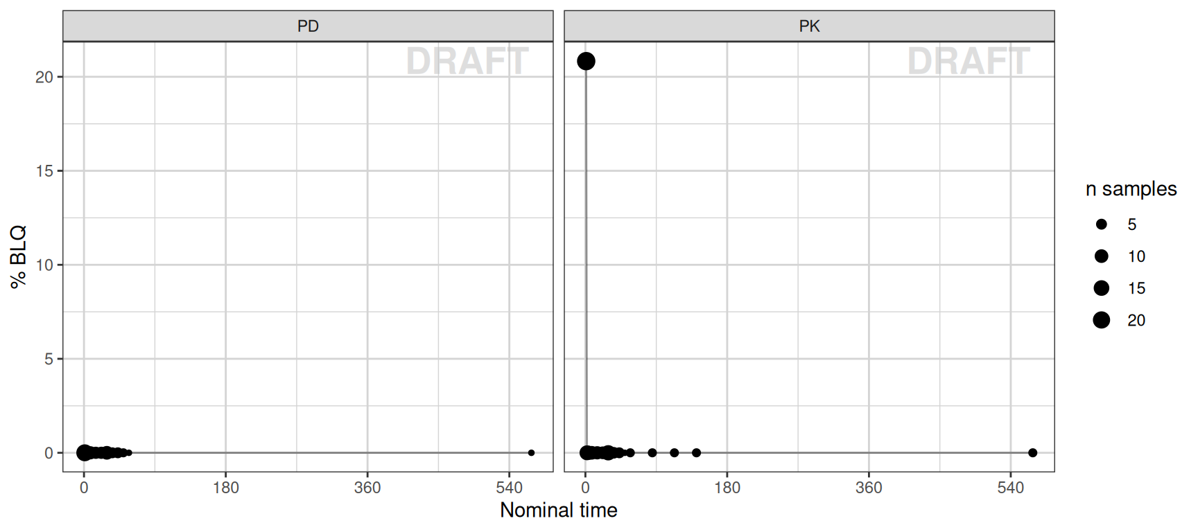

blq_by_dose <- blq %>%
  group_by(NAME, TRT_low2high) %>%
  summarise(
    n_obs = n(),
    pct_blq = round(100 * mean(is_blq, na.rm = TRUE), 1),
    .groups = "drop"
  )

datatable(blq_by_dose, caption = "BLQ fraction by treatment arm")

Dose and PK/PD Data Collection Times

Overview of the timing of dose, PK, and PD collection for all patients. Each “x” is a record (a dose time or an assessment time). Each red circle flags a possible dose interruption, when the gap between doses exceeds DT_flag and NAME == NAME_DOSE. Adjust fig.height/fig.width for larger datasets.

DT_flag <- 10 # > DT_flag days between doses is flagged
NAME_DOSE <- "Dose" # NAME == NAME_DOSE is flagged

data_dose_interruption <- data %>%
  group_by(USUBJID, NAME) %>%
  mutate(DT = lead(TIME, default = max(TIME)) - TIME, TMID = TIME + DT / 2) %>%
  ungroup() %>%
  filter(DT > DT_flag, NAME == NAME_DOSE)

ggplot(data, aes(x = TIME, y = USUBJID)) +
  geom_point(shape = 4) +
  geom_point(
    data = data_dose_interruption,
    aes(x = TMID, y = USUBJID),
    color = "red",
    alpha = 0.2,
    size = 5
  ) +
  xgx_scale_x_time_units(units_dataset = time_units_dataset) +
  facet_wrap(~ YTYPE + NAME, labeller = label_both)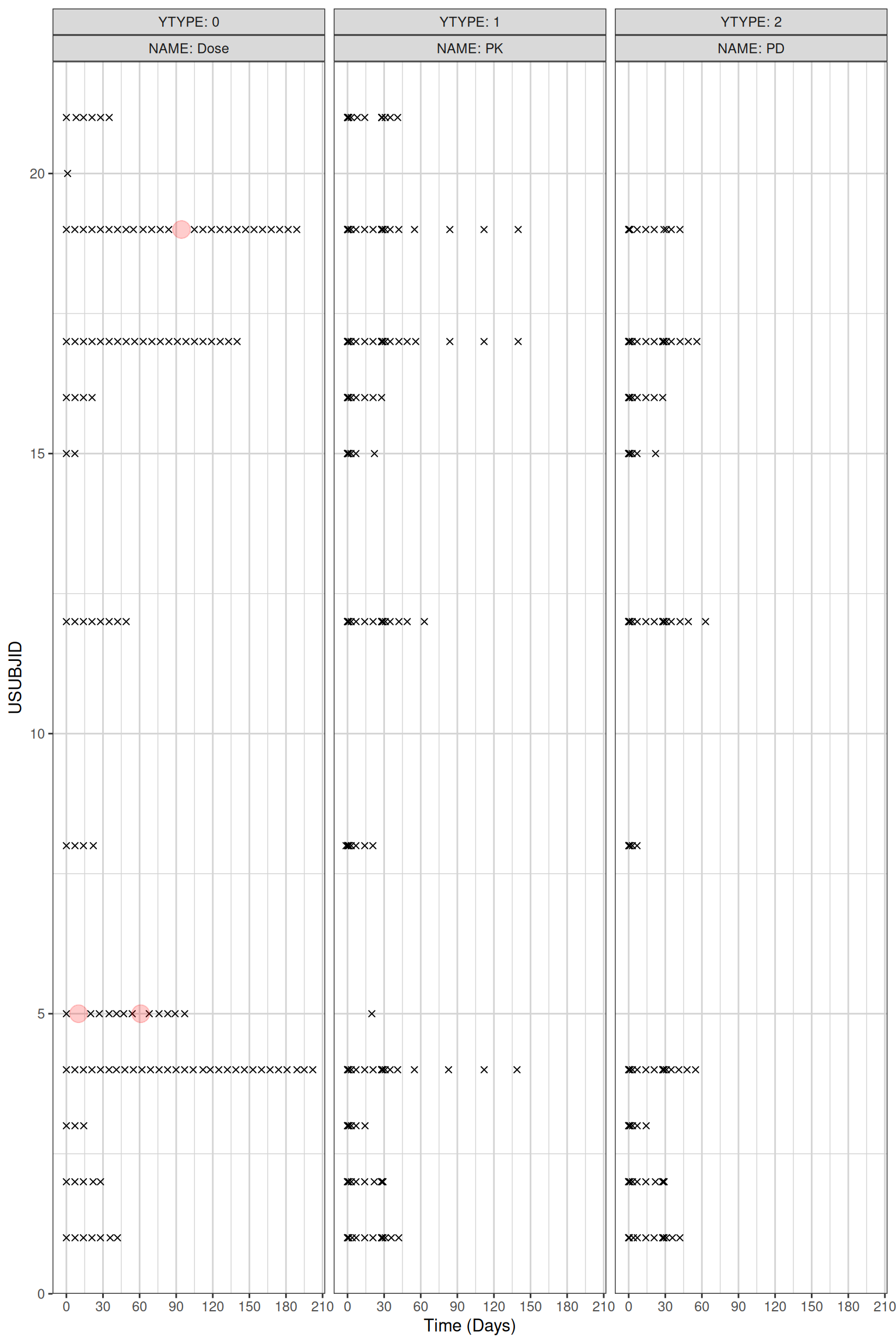

Nominal vs Actual Time Discrepancies

A common error is that either the nominal or actual time was derived incorrectly. Points that don’t lie near the identity line need investigation.

xymin <- min(c(data$NOMTIME, data$TIME), na.rm = TRUE)
xymax <- max(c(data$NOMTIME, data$TIME), na.rm = TRUE)

ggplot(data, aes(x = TIME, y = NOMTIME)) +
  geom_point() +
  annotate(
    "segment",
    x = xymin,
    xend = xymax,
    y = xymin,
    yend = xymax,
    color = "blue"
  ) +
  xlim(c(xymin, xymax)) +
  ylim(c(xymin, xymax))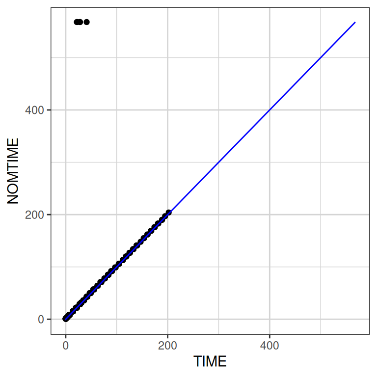

# Rounded: NOMTIME - TIME is a floating-point subtraction, so an exact 3.08
# prints as 3.079999999999998 and swamps the column. Named time_discrepancy
# rather than difftime, which would shadow base::difftime().
time_discrepancy <- data %>%
  mutate(DIFF_TIME = round(abs(NOMTIME - TIME), 2)) %>%
  arrange(-DIFF_TIME) %>%
  slice(1:10) %>%
  select(USUBJID, TRT, DIFF_TIME, TIME, NOMTIME, YTYPE, NAME, LIDV)

datatable(time_discrepancy)

Unique Nominal Time Values

Check the nominal times to make sure they’re correct (e.g. that hour-scale values weren’t accidentally set equal to day-scale values).

sort(unique(data$NOMTIME))

##  [1]   1   2   4   8  15  22  29  30  32  36  43  50  57  64  71  78  85  92  99
## [20] 106 113 120 127 134 141 148 155 162 169 176 183 190 197 204 568

Missing Data

Understand what is absent: how much data is missing, which columns it affects, whether variables tend to be missing together, and whether missingness appears related to other variables. Missingness drives modeling decisions (imputation, dropping subjects, or restructuring the analysis), so it gets its own section.

Columns that Contain NAs

A modeling dataset often is not supposed to contain any NAs. This table highlights where they occur. If it is empty, there are no NAs.

na_summary <- data %>%
  dplyr::summarise_all(function(x) sum(is.na(x))) %>%
  t() %>%
  as.data.frame() %>%
  rename(N_NA = V1)
na_summary$Column <- names(data)
na_summary <- na_summary %>%
  select(Column, N_NA) %>%
  filter(N_NA > 0)

datatable(na_summary)

Missing-data patterns

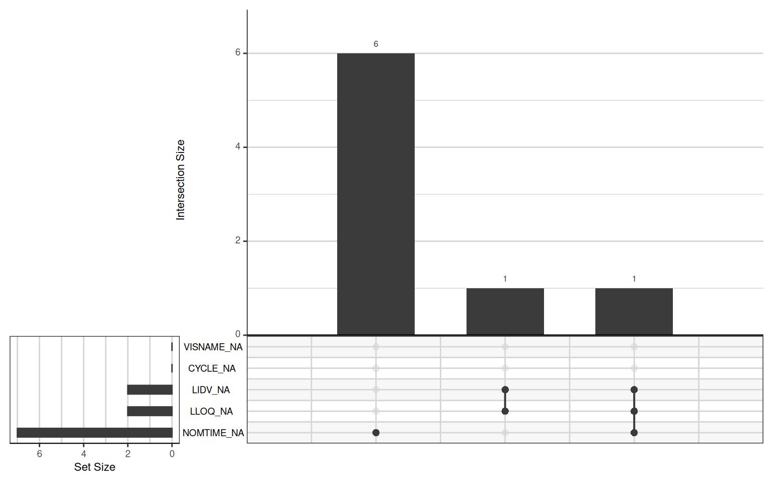
The table above says how much is missing per column. This says which variables tend to be missing together, which is the more useful question — missingness that clusters usually points at one upstream cause (a visit not done, a sample lost) rather than many independent ones.

gg_miss_upset from the naniar package draws that. If no combinations of missing values exist the plot is empty or errors, so it is wrapped in try() and the rest of the document still renders.

if (any(is.na(data1))) {
  try(print(naniar::gg_miss_upset(data1)))
} else {
  cat("No missing values in the per-subject data.\n")
}

Possible missingness mechanism

To probe whether missingness is related to observed variables (a step toward distinguishing missing-completely-at-random from missing-at-random), compare the covariates between subjects who are missing vs. not missing a chosen variable. Set missingness_target to a variable of interest. This is descriptive only — it flags associations to investigate, not a formal test.

# EDIT THIS: variable whose missingness you want to characterize.
missingness_target <- intersect(covariates, names(data1))[1]

if (!is.na(missingness_target) && any(is.na(data1[[missingness_target]]))) {
  data1 %>%
    mutate(
      .is_missing = ifelse(
        is.na(.data[[missingness_target]]),
        "missing",
        "observed"
      )
    ) %>%
    select(.is_missing, any_of(covariates)) %>%
    select(.is_missing, where(is.numeric)) %>%
    pivot_longer(-.is_missing) %>%
    group_by(name, .is_missing) %>%
    summarise(
      n = sum(!is.na(value)),
      median = median(value, na.rm = TRUE),
      Q1 = quantile(value, 0.25, na.rm = TRUE),
      Q3 = quantile(value, 0.75, na.rm = TRUE),
      .groups = "drop"
    ) %>%
    datatable(
      caption = paste("Covariates by missingness of", missingness_target)
    )
} else {
  cat("No missing values in the selected target, or no target available.\n")
}

## No missing values in the selected target, or no target available.

Distributions and Relationships

Screen the covariates themselves — their distributions and how they relate to one another — to flag issues to address before modeling:

• Skewed data: consider transforming before regression.
• Outliers: consider removal, down-weighting, or a closer look.
• Small categories: consider grouping if numbers are too small to power an effect.
• Highly correlated variables: consider using only one in a regression.

Covariate Summary

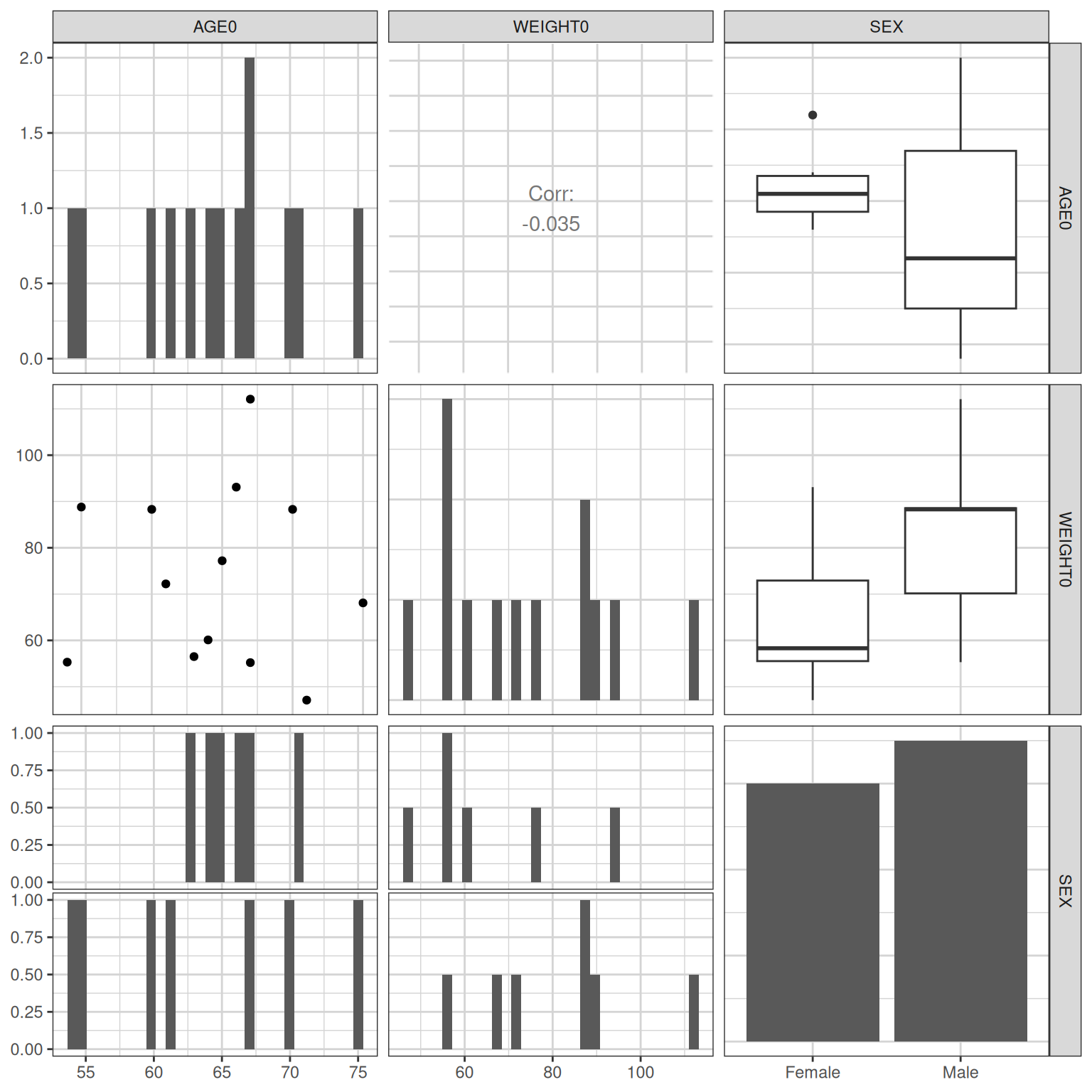
Numerical summary of the covariates: quartiles for continuous variables and level counts for categorical ones, followed by a pairs plot.

The pairs plot carries the whole picture on its own — the diagonal gives each variable’s distribution (so skew and outliers are visible there), and the off-diagonal panels give every pairwise relationship. Separate histograms and bar charts of the same variables would only repeat the diagonal, so there are none.

# Split covariates once, here, and reuse the split everywhere below. A variable
# is treated as continuous only if it is numeric AND takes enough distinct
# values to be worth summarising as one -- a 0/1 numeric flag is categorical
# however it is stored.
num_unique_vals <- data1[, covariates] %>%
  summarise_all(function(x) length(unique(x))) %>%
  as.numeric()
is_numeric_cov <- vapply(data1[, covariates, drop = FALSE], is.numeric, logical(1))

cts_names <- covariates[is_numeric_cov & num_unique_vals >= 8]
cat_names <- setdiff(covariates, cts_names)

cts_cov <- data1 |> select(all_of(cts_names))
cat_cov <- data1 |> select(all_of(cat_names))

cts_cov_summary <- cts_cov %>%
  pivot_longer(everything()) %>%
  group_by(name) %>%
  summarise(
    n_missing_or_NA = sum(is.na(value)),
    min = min(value, na.rm = TRUE),
    Q1 = quantile(value, 0.25, na.rm = TRUE),
    median = median(value, na.rm = TRUE),
    Q3 = quantile(value, 0.75, na.rm = TRUE),
    max = max(value, na.rm = TRUE)
  ) %>%
  # round summary stats to 3 significant digits (handles any magnitude,
  # no forced scientific notation); leave the integer count alone
  mutate(across(c(min, Q1, median, Q3, max), ~ signif(.x, 3)))
datatable(cts_cov_summary)

cat_summary <- function(x) {
  unique_x <- sort(unique(x))
  str <- 1:length(unique_x)
  for (i in 1:length(unique_x)) {
    str[i] <- paste0(unique_x[i], "=", sum(x == unique_x[i], na.rm = TRUE))
  }
  paste(str, collapse = ", ")
}

cat_cov_summary <- cat_cov %>%
  pivot_longer(everything()) %>%
  group_by(name) %>%
  summarise(
    n_missing_or_NA = sum(is.na(value)),
    n_distinct = n_distinct(value),
    count_summary = cat_summary(value)
  )
datatable(cat_cov_summary)

GGally::ggpairs(
  data1,
  columns = covariates,
  diag = list(continuous = "barDiag")
)

Correlations: Correlated Variables

Watch for high correlations (> 0.4); for those, consider using only one in any covariate analysis. This uses Spearman’s rank correlation, which works with both continuous and categorical (factor-coded) values.

# Categorical covariates are factor-coded to numbers so Spearman can rank them.
cat_cov_num <- cat_cov %>%
  mutate(across(everything(), ~ as.numeric(factor(.))))

data_cov_all_num <- bind_cols(cts_cov, cat_cov_num)

M <- cor(data_cov_all_num, method = "spearman", use = "pairwise.complete.obs")
corrplot::corrplot.mixed(M, lower = "number", upper = "ellipse")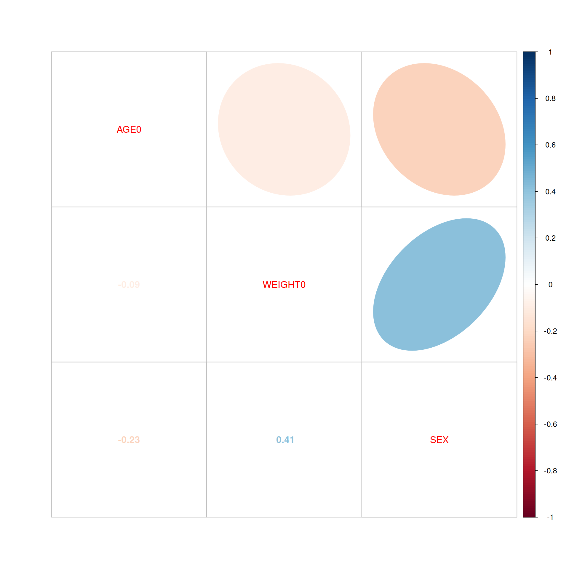

Largest Correlations

Mupper <- M
Mupper[lower.tri(M, diag = TRUE)] <- 0

n_largest <- 3 # always show the n largest correlations
corr_threshold <- 0.4 # also show all correlations above this threshold

# as.data.frame.table() turns the correlation matrix into one row per pair with
# Var1/Var2/corr columns. That is what the reshape2 melt() call here used to do;
# base R does it with no dependency, and reshape2 is superseded by tidyr anyway.
largest_corr <- Mupper %>%
  as.data.frame.table(responseName = "corr", stringsAsFactors = FALSE) %>%
  filter(abs(corr) > 0) %>%
  arrange(-abs(corr)) %>%
  mutate(n = 1:n()) %>%
  filter(n <= n_largest | abs(corr) > corr_threshold)

knitr::kable(largest_corr, caption = "Largest correlations", digits = 2)

Largest correlations

Var1	Var2	corr	n
WEIGHT0	SEX	0.41	1
AGE0	SEX	-0.23	2
AGE0	WEIGHT0	-0.09	3

The pairs plot in Covariate Summary already shows these pairs jointly, so the table is the addition here: it names and ranks them rather than leaving you to read them off a grid.

Overview of Entire Dataset

A more complete overview of every column in the dataset using Hmisc.

data1 %>%
  Hmisc::describe() %>%
  Hmisc::html(size = 80)

.

31 Variables   13 Observations

---

STUDYID

n	missing	distinct	value
13	0	1	CABC123A12101

 Value      CABC123A12101
 Frequency             13
 Proportion             1 

---

ID

n	missing	distinct	Info	Mean	pMedian	Gmd	.05	.10	.25	.50	.75	.90	.95
13	0	13	1	11	11	8.769	1.6	2.2	4.0	12.0	17.0	19.8	20.4

 Value          1     2     3     4     5     8    12    15    16    17    19    20
 Frequency      1     1     1     1     1     1     1     1     1     1     1     1
 Proportion 0.077 0.077 0.077 0.077 0.077 0.077 0.077 0.077 0.077 0.077 0.077 0.077
                 
 Value         21
 Frequency      1
 Proportion 0.077 

---

USUBJID

n	missing	distinct	Info	Mean	pMedian	Gmd	.05	.10	.25	.50	.75	.90	.95
13	0	13	1	11	11	8.769	1.6	2.2	4.0	12.0	17.0	19.8	20.4

 Value          1     2     3     4     5     8    12    15    16    17    19    20
 Frequency      1     1     1     1     1     1     1     1     1     1     1     1
 Proportion 0.077 0.077 0.077 0.077 0.077 0.077 0.077 0.077 0.077 0.077 0.077 0.077
                 
 Value         21
 Frequency      1
 Proportion 0.077 

---

TIME

        n  missing distinct     Info     Mean  pMedian      Gmd      .05      .10 
       13        0       12    0.997 -0.06615    -0.06   0.3721   -0.560   -0.132 
      .25      .50      .75      .90      .95 
   -0.090   -0.070   -0.020   -0.002    0.400  

 Value      -1.19 -0.14 -0.10 -0.09 -0.08 -0.07 -0.05 -0.04 -0.02 -0.01  0.00  1.00
 Frequency      1     1     1     1     1     2     1     1     1     1     1     1
 Proportion 0.077 0.077 0.077 0.077 0.077 0.154 0.077 0.077 0.077 0.077 0.077 0.077 

---

NOMTIME

n	missing	distinct	Info	Mean
6	7	2	0.429	1.167

 Value          1     2
 Frequency      5     1
 Proportion 0.833 0.167 

---

TIMEUNIT

n	missing	distinct	value
13	0	1	Days

 Value      Days
 Frequency    13
 Proportion    1 

---

AMT

n	missing	distinct	Info	Mean	pMedian	Gmd
13	0	3	0.396	4.615	0	8.923

 Value          0    12    48
 Frequency     11     1     1
 Proportion 0.846 0.077 0.077 

---

LIDV

n	missing	distinct	Info	Mean	pMedian	Gmd	.05	.10	.25	.50	.75	.90	.95
11	2	11	1	15.22	16.17	9.129	7.740	7.904	8.482	11.293	23.811	25.930	26.761

 Value       7.577  7.904  8.305  8.660 10.622 11.293 11.865 23.019 24.603 25.930
 Frequency       1      1      1      1      1      1      1      1      1      1
 Proportion  0.091  0.091  0.091  0.091  0.091  0.091  0.091  0.091  0.091  0.091
                  
 Value      27.593
 Frequency       1
 Proportion  0.091 

---

YTYPE

n	missing	distinct	Info	Sum	Mean
13	0	2	0.393	11	0.8462

---

ADM

n	missing	distinct	Info	Sum	Mean
13	0	2	0.393	2	0.1538

---

CMT

n	missing	distinct	Info	Sum	Mean
13	0	2	0.393	11	0.8462

---

NAME

n	missing	distinct
13	0	2

 Value       Dose    PK
 Frequency      2    11
 Proportion 0.154 0.846 

---

EVENTU

n	missing	distinct
13	0	2

 Value         mg ng/mL
 Frequency      2    11
 Proportion 0.154 0.846 

---

UNIT

n	missing	distinct
13	0	2

 Value         mg ng/mL
 Frequency      2    11
 Proportion 0.154 0.846 

---

MDV

n	missing	distinct	Info	Sum	Mean
13	0	2	0.393	2	0.1538

---

CENS

n	missing	distinct	Info	Sum	Mean
13	0	2	0.393	11	0.8462

---

EVID

n	missing	distinct	Info	Sum	Mean
13	0	2	0.393	2	0.1538

---

AGEB

n	missing	distinct	Info	Mean	pMedian	Gmd	.05	.10	.25	.50	.75	.90	.95
13	0	12	0.997	64.46	65	7.026	54.6	56.0	61.0	65.0	67.0	70.8	72.6

 Value         54    55    60    61    63    64    65    66    67    70    71    75
 Frequency      1     1     1     1     1     1     1     1     2     1     1     1
 Proportion 0.077 0.077 0.077 0.077 0.077 0.077 0.077 0.077 0.154 0.077 0.077 0.077 

---

AGE0

n	missing	distinct	Info	Mean	pMedian	Gmd	.05	.10	.25	.50	.75	.90	.95
13	0	12	0.997	64.46	65	7.026	54.6	56.0	61.0	65.0	67.0	70.8	72.6

 Value         54    55    60    61    63    64    65    66    67    70    71    75
 Frequency      1     1     1     1     1     1     1     1     2     1     1     1
 Proportion 0.077 0.077 0.077 0.077 0.077 0.077 0.077 0.077 0.154 0.077 0.077 0.077 

---

WEIGHTB

        n  missing distinct     Info     Mean  pMedian      Gmd      .05      .10 
       13        0       12    0.997    74.02    72.65    22.42    51.96    55.22 
      .25      .50      .75      .90      .95 
    56.50    72.20    88.30    92.24   100.70  

 Value       47.1  55.2  55.3  56.5  60.1  68.1  72.2  77.2  88.3  88.8  93.1 112.1
 Frequency      1     1     1     1     1     1     1     1     2     1     1     1
 Proportion 0.077 0.077 0.077 0.077 0.077 0.077 0.077 0.077 0.154 0.077 0.077 0.077 

---

WEIGHT0

        n  missing distinct     Info     Mean  pMedian      Gmd      .05      .10 
       13        0       12    0.997    74.02    72.65    22.42    51.96    55.22 
      .25      .50      .75      .90      .95 
    56.50    72.20    88.30    92.24   100.70  

 Value       47.1  55.2  55.3  56.5  60.1  68.1  72.2  77.2  88.3  88.8  93.1 112.1
 Frequency      1     1     1     1     1     1     1     1     2     1     1     1
 Proportion 0.077 0.077 0.077 0.077 0.077 0.077 0.077 0.077 0.154 0.077 0.077 0.077 

---

SEXN

n	missing	distinct	Info	Mean
13	0	2	0.75	1.462

 Value          1     2
 Frequency      7     6
 Proportion 0.538 0.462 

---

SEX

n	missing	distinct
13	0	2

 Value      Female   Male
 Frequency       6      7
 Proportion  0.462  0.538 

---

TRTN

n	missing	distinct	Info	Mean	pMedian	Gmd
13	0	5	0.929	26.08	27	21.54

 Value          3     6    12    24    48
 Frequency      1     2     3     2     5
 Proportion 0.077 0.154 0.231 0.154 0.385 

---

TRT

n	missing	distinct
13	0	5

 Value      12 mg 24 mg  3 mg 48 mg  6 mg
 Frequency      3     2     1     5     2
 Proportion 0.231 0.154 0.077 0.385 0.154 

---

PROFDAY

n	missing	distinct	Info	Mean
13	0	1	0	0

 Value       0
 Frequency  13
 Proportion  1 

---

VISNAME

n	missing	distinct
13	0	2

 Value      CYCLE 1 DAY 1 CYCLE 1 DAY 2
 Frequency             12             1
 Proportion         0.923         0.077 

---

CYCLE

n	missing	distinct	Info	Mean
13	0	1	0	1

 Value       1
 Frequency  13
 Proportion  1 

---

LLOQ

n	missing	distinct	Info	Mean
11	2	1	0	10

 Value      10
 Frequency  11
 Proportion  1 

---

TRT_low2high

n	missing	distinct
13	0	5

 Value       3 mg  6 mg 12 mg 24 mg 48 mg
 Frequency      1     2     3     2     5
 Proportion 0.077 0.154 0.231 0.154 0.385 

---

TRT_high2low

n	missing	distinct
13	0	5

 Value      48 mg 24 mg 12 mg  6 mg  3 mg
 Frequency      5     2     3     2     1
 Proportion 0.385 0.154 0.231 0.154 0.077 

---

Portable Summary Export

Write a machine- and human-readable summary of the checks in this document to disk, so it can be moved to another machine and reviewed (by a person or an AI) alongside the code. Two files are produced:

• _*_summary_full.json — fully informative and unmasked. Includes real study IDs, counts, true min/max, and the specific USUBJIDs that triggered each failed check (so issues can be traced back and fixed). This file contains subject identifiers; keep it local.
• _*_summary_no_subjids.json — identical to the full file, but with every USUBJID removed (offending-subject lists collapsed to counts). Everything else — study IDs, counts, min/max — is retained. Safer to share when subject identifiers should not leave the environment.

Both names start with an underscore deliberately. If this document is rendered as part of an R Markdown site, render_site() copies loose files in the source directory into the published output, and .json is not one of the extensions it excludes — but anything beginning with _ is. Without the underscore, the unmasked export would be published to the website.

# offending subjects per failed check (used only in the full export) -----------

# continuous plausibility violations: which subjects, which value
offending_continuous <- plausibility_ranges %>%
  filter(variable %in% names(data)) %>%
  purrr::pmap(function(variable, lower, upper) {
    x <- data[[variable]]
    idx <- !is.na(x) & (x < lower | x > upper)
    if (!any(idx)) {
      return(NULL)
    }
    data[idx, ] %>%
      transmute(
        USUBJID,
        STUDYID,
        variable = variable,
        value = .data[[variable]],
        lower = lower,
        upper = upper
      )
  }) %>%
  bind_rows()

# unexpected categorical levels: which subjects, which value
offending_categorical <- purrr::imap(allowed_levels, function(allowed, var) {
  if (!var %in% names(data)) {
    return(NULL)
  }
  x <- data[[var]]
  idx <- !is.na(x) & !(x %in% allowed)
  if (!any(idx)) {
    return(NULL)
  }
  data[idx, ] %>%
    transmute(
      USUBJID,
      STUDYID,
      variable = var,
      value = as.character(.data[[var]])
    )
}) %>%
  bind_rows()

# duplicate USUBJID/TIME records
offending_duplicate_times <- data %>%
  group_by(USUBJID, TIME) %>%
  filter(n() > 1) %>%
  ungroup() %>%
  transmute(USUBJID, STUDYID, TIME, YTYPE, NAME)

# negative or zero dependent variable among observations
offending_dv <- data %>%
  filter(EVID == 0, !is.na(LIDV), LIDV <= 0) %>%
  transmute(USUBJID, STUDYID, TIME, YTYPE, NAME, LIDV)

# assemble the full (unmasked) summary ----------------------------------------
summary_full <- list(
  provenance = list(
    source_file = normalizePath(filename, mustWork = FALSE),
    file_last_modified = as.character(file.info(filename)$mtime),
    report_run_at = format(Sys.time(), "%Y-%m-%d %H:%M"),
    n_rows = nrow(data),
    n_columns = ncol(data),
    n_subjects = dplyr::n_distinct(data$USUBJID),
    studies = sort(unique(data$STUDYID))
  ),
  n_subjects_by_study_arm = summary_by_trt,
  n_datapoints_by_study_arm_ytype = summary_by_trt_ytype,
  na_counts_by_column = na_summary,
  offending = list(
    continuous_plausibility = offending_continuous,
    categorical_unexpected = offending_categorical,
    duplicate_times = offending_duplicate_times,
    nonpositive_dv = offending_dv
  ),
  offending_counts = list(
    continuous_plausibility = nrow(offending_continuous),
    categorical_unexpected = nrow(offending_categorical),
    duplicate_times = nrow(offending_duplicate_times),
    nonpositive_dv = nrow(offending_dv)
  )
)

# derive the masked summary by stripping USUBJIDs -----------------------------
# The mask is a transform of the full summary, so there is a single source of
# truth. Offending-subject lists are collapsed to counts; everything else stays.
strip_usubjid <- function(x) {
  if (is.data.frame(x)) {
    return(x[, setdiff(names(x), "USUBJID"), drop = FALSE])
  }
  if (is.list(x)) {
    return(lapply(x, strip_usubjid))
  }
  x
}

summary_no_subjids <- summary_full
# replace the detailed offending lists with counts only, then strip any stray IDs
summary_no_subjids$offending <- summary_full$offending_counts
summary_no_subjids <- strip_usubjid(summary_no_subjids)

# write both files next to the rendered document ------------------------------
#
# The leading underscore is load-bearing, not cosmetic. rmarkdown::render_site()
# copies every file in this directory into the published site except dotfiles,
# *_cache, a fixed list of source extensions, and anything starting with "_".
# .json is NOT on that exclusion list, so without the underscore the unmasked
# export -- the one holding USUBJIDs -- would be published alongside the page.
out_stem <- paste0("_", str_replace(Rmd_name, "\\.Rmd$", ""))
path_full <- paste0(out_stem, "_summary_full.json")
path_masked <- paste0(out_stem, "_summary_no_subjids.json")

jsonlite::write_json(
  summary_full,
  path_full,
  auto_unbox = TRUE,
  pretty = TRUE,
  na = "null"
)
jsonlite::write_json(
  summary_no_subjids,
  path_masked,
  auto_unbox = TRUE,
  pretty = TRUE,
  na = "null"
)

cat(
  "Wrote:\n ",
  path_full,
  " (unmasked, contains USUBJIDs)\n ",
  path_masked,
  " (no subject IDs)\n",
  sep = ""
)

## Wrote:
##  _Data_Checking_summary_full.json (unmasked, contains USUBJIDs)
##  _Data_Checking_summary_no_subjids.json (no subject IDs)

Summarize Findings

Summarize what the checks above revealed, so anyone reading the report can see the state of the data at a glance. The goal here is to describe what was found, not to decide how it changes the modeling — that decision belongs to the analysis plan, not this document. Fill this in each time you run the file.

• Data quality issues found: (e.g. out-of-range weights, duplicate times, undocumented columns)
• Missing data: (extent, patterns, and apparent mechanism)
• Distributions: (skewed variables that may need transformation before modeling)
• Outliers: (any, and whether they warrant a closer look)
• Small categories: (any levels with very few subjects)
• Correlated covariates: (pairs above threshold)

Future Enhancements (Parking Lot)

Ideas to strengthen this workflow, deferred for now. Kept here so they survive into the template and are not forgotten. None are required for the document to be useful today.

Adopt mature data-quality tooling instead of bespoke checks. The plausibility and validity checks here could be replaced or backed by established R packages, which bring tested logic and standard reporting:

• NMdata — the pharmacometrics-specific one, and the closest fit to this document. NMcheckData() runs an automated battery against the conventions NONMEM enforces: TIME non-decreasing within a subject, AMT/EVID/MDV/DV agreement, CMT validity, ADDL/II/SS/RATE rules, duplicate events on ID+CMT+EVID+TIME, subject-invariant covariates, and ID/USUBJID correspondence. The Dataset Integrity Checks section above is modelled on that list. Adopting the package outright would tie this document to NONMEM conventions and to a single-maintainer dependency, which is why the checks are written out here instead — but if your workflow is NONMEM-based, use it directly.
• pointblank — declarative data validation: state expectations (ranges, allowed values, uniqueness) and get a pass/fail report. A natural fit for the “Checking Values Are Valid” section. Domain-agnostic: it knows nothing about EVID or compartments.
• dataquieR — the STRATOS-lineage data-quality framework; a more formal, comprehensive take on the same IDA activities in this document. Also domain-agnostic.
• apmx — the upstream counterpart to NMdata: automated assembly of popPK/PKPD datasets from SDTM or ADaM, where pk_build() warns and flags records that would stop NONMEM estimating. Worth considering if datasets are being assembled rather than handed over — one builds a correct dataset, the other checks one you were given.

Check the dataset against its specification. Every check in this document compares the data against expectations written inside the document — plausibility_ranges, allowed_levels, subject_invariant. The check not being done is the one against the dataset’s own spec: are all the documented columns present, are there columns nobody documented, do the types and units match what the spec claims, are the derived columns actually derived that way. This is the “data specification matching” step in DataCheQC (Dotan, Radivojevic & Singh, CPT:PSP 2023), and it is the largest remaining gap here.

The reason it is parked rather than written is that specification formats are company-specific — a Word table, an Excel define sheet, a CDISC define.xml, or (as in this repository) a Markdown table in Data/*.md. Any parser written here would fit exactly one of those and break on the rest, which is why a general-purpose implementation is the wrong shape for a template.

That makes it a natural fit for the agent described below: reading a heterogeneous spec document, aligning it to a data frame, and reporting mismatches is the kind of task an LLM handles well and a regex does not. Treat the spec as an input to the reviewer agent rather than as another chunk of R.

Turn the exported summary into an AI-assisted review. The Portable Summary Export already writes a machine-readable artifact. That is the input contract for a future “data-cleaning reviewer” agent that reads the summary and this code, flags weaknesses, and drafts the Summary of Findings. Relevant building blocks:

• ellmer — R-native LLM interface (tool use, structured output); the natural harness for such a reviewer in R.
• btw — supplies R session/data context to an LLM.
• ISoP AI/ML SIG Agentic Workflows (glossary, PMbench leaderboard) — the community effort to evaluate and standardize PMX agents, worth aligning with or contributing back to.

When picking any of these up: vet the current scope and activity of each package/repo first (this space moves quickly), and keep the human-in-the-loop — an AI reviewer should draft findings for a modeler to adjudicate, never sign off.

References

Pharmacometrics

• Byon W, Smith MK, Chan P, Tortorici MA, Riley S, Dai H, Dong J, Ruiz-Garcia A, Sweeney K, Cronenberger C (2013). Establishing best practices and guidance in population modeling: an experience with an internal population pharmacokinetic analysis guidance. CPT Pharmacometrics Syst Pharmacol 2(7): e51. https://doi.org/10.1038/psp.2013.26
• U.S. Food and Drug Administration (2022). Population Pharmacokinetics: Guidance for Industry. https://www.fda.gov/regulatory-information/search-fda-guidance-documents/population-pharmacokinetics — sets the expectation that data handling, BLQ treatment, outliers and missing data are described in the analysis.
• Bergstrand M, Karlsson MO (2009). Handling data below the limit of quantification in mixed effect models. AAPS J 11(2): 371–380. https://doi.org/10.1208/s12248-009-9112-5 — the M1–M4 comparison behind the BLQ section.
• Beal SL (2001). Ways to fit a PK model with some data below the quantification limit. J Pharmacokinet Pharmacodyn 28(5): 481–504. https://doi.org/10.1023/A:1012299115260 — the original enumeration of the M1–M7 methods.
• Delff P. NMdata: preparation, checking and post-processing data for PK/PD modeling. https://cran.r-project.org/package=NMdata — NMcheckData() is the reference implementation of the dataset integrity checks used here.

Initial data analysis and data quality

• Baillie M, le Cessie S, Schmidt CO, Lusa L, Huebner M, for the STRATOS Initiative (2022). Ten simple rules for initial data analysis. PLoS Comput Biol 18(2): e1009819. https://doi.org/10.1371/journal.pcbi.1009819
• Huebner M, le Cessie S, Schmidt CO, Vach W (2018). A contemporary conceptual framework for initial data analysis. Observational Studies 4: 171–192. https://doi.org/10.1353/obs.2018.0014
• Huebner M, Vach W, le Cessie S, Schmidt CO, Lusa L (2020). Hidden analyses: a review of reporting practice and recommendations for more transparent reporting of initial data analyses. BMC Med Res Methodol 20: 61. https://doi.org/10.1186/s12874-020-00942-y
• Chatfield C (1985). The initial examination of data. J R Stat Soc Ser A 148(3): 214–253. https://doi.org/10.2307/2981969
• Lee KJ, Tilling KM, Cornish RP, et al. (2021). Framework for the treatment and reporting of missing data in observational studies (TARMOS). J Clin Epidemiol 134: 79–88. https://doi.org/10.1016/j.jclinepi.2021.01.008
• Schmidt CO, Struckmann S, Enzenbach C, et al. (2021). Facilitating harmonized data quality assessments: a data quality framework for observational health research data collections with software implementations in R (dataquieR). BMC Med Res Methodol 21: 63. https://doi.org/10.1186/s12874-021-01252-7
• Vandemeulebroecke M, Baillie M, Margolskee A, Magnusson B (2019). Effective visual communication for the quantitative scientist. CPT Pharmacometrics Syst Pharmacol 8: 705–719. https://doi.org/10.1002/psp4.12455

R Session Info

sessionInfo()

## R version 4.6.1 (2026-06-24)
## Platform: x86_64-pc-linux-gnu
## Running under: Ubuntu 24.04.4 LTS
## 
## Matrix products: default
## BLAS:   /usr/lib/x86_64-linux-gnu/openblas-pthread/libblas.so.3 
## LAPACK: /usr/lib/x86_64-linux-gnu/openblas-pthread/libopenblasp-r0.3.26.so;  LAPACK version 3.12.0
## 
## locale:
##  [1] LC_CTYPE=C.UTF-8       LC_NUMERIC=C           LC_TIME=C.UTF-8       
##  [4] LC_COLLATE=C.UTF-8     LC_MONETARY=C.UTF-8    LC_MESSAGES=C.UTF-8   
##  [7] LC_PAPER=C.UTF-8       LC_NAME=C              LC_ADDRESS=C          
## [10] LC_TELEPHONE=C         LC_MEASUREMENT=C.UTF-8 LC_IDENTIFICATION=C   
## 
## time zone: UTC
## tzcode source: system (glibc)
## 
## attached base packages:
## [1] stats     graphics  grDevices utils     datasets  methods   base     
## 
## other attached packages:
##  [1] GGally_2.4.0    DT_0.34.0       lubridate_1.9.5 forcats_1.0.1  
##  [5] stringr_1.6.0   purrr_1.2.2     readr_2.2.0     tibble_3.3.1   
##  [9] tidyverse_2.0.0 xgxr_1.1.6      zoo_1.9-0       gridExtra_2.3.1
## [13] tidyr_1.3.2     dplyr_1.2.1     ggplot2_4.0.3  
## 
## loaded via a namespace (and not attached):
##  [1] tidyselect_1.2.1   Exact_3.3          rootSolve_1.8.2.4  farver_2.1.2      
##  [5] S7_0.2.2           bitops_1.1-0       fastmap_1.2.0      RCurl_1.98-1.19   
##  [9] digest_0.6.39      rpart_4.1.27       timechange_0.4.0   lifecycle_1.0.5   
## [13] Deriv_4.3.0        cluster_2.1.8.2    lmom_3.3           magrittr_2.0.5    
## [17] compiler_4.6.1     rlang_1.3.0        Hmisc_5.2-6        sass_0.4.10       
## [21] tools_4.6.1        corrplot_0.95      yaml_2.3.12        data.table_1.18.4 
## [25] knitr_1.51         labeling_0.4.3     htmlwidgets_1.6.4  plyr_1.8.9        
## [29] RColorBrewer_1.1-3 expm_1.0-0         withr_3.0.3        foreign_0.8-91    
## [33] nnet_7.3-20        grid_4.6.1         e1071_1.7-17       colorspace_2.1-3  
## [37] scales_1.4.0       MASS_7.3-65        cli_3.6.6          mvtnorm_1.4-2     
## [41] UpSetR_1.4.1       rmarkdown_2.31     generics_0.1.4     otel_0.2.0        
## [45] rstudioapi_0.19.0  binom_1.1-2        httr_1.4.8         tzdb_0.5.0        
## [49] readxl_1.5.0       gld_2.6.8          cachem_1.1.0       proxy_0.4-29      
## [53] pander_0.6.6       assertthat_0.2.1   cellranger_1.1.0   base64enc_0.1-6   
## [57] vctrs_0.7.3        boot_1.3-32        Matrix_1.7-5       minpack.lm_1.2-4  
## [61] jsonlite_2.0.0     naniar_1.1.0       hms_1.1.4          visdat_0.6.0      
## [65] Formula_1.2-6      htmlTable_2.5.0    crosstalk_1.2.2    jquerylib_0.1.4   
## [69] glue_1.8.1         ggstats_0.13.0     stringi_1.8.9      gtable_0.3.6      
## [73] pillar_1.11.1      htmltools_0.5.9    R6_2.6.1           evaluate_1.0.5    
## [77] lattice_0.22-9     haven_2.5.5        png_0.1-9          backports_1.5.1   
## [81] bslib_0.12.0       class_7.3-23       DescTools_0.99.60  Rcpp_1.1.2        
## [85] checkmate_2.3.4    xfun_0.60          fs_2.1.0           pkgconfig_2.0.3