PD - Multiple Ascending Dose - Realistic Data
Alison Margolskee, Kostas Biliouris
Overview
This document contains PD exploratory graphs and also the R code that generates these graphs. The plots presented here are inspired by a real study which involved multiple types of PD data, from continuous endpoints to ordinal response and count data.
This code makes use of the following files which can be downloaded from the available links
Data specifications can be accessed on Datasets and Rmarkdown template to generate this page can be found on Rmarkdown-Template.
Setup
# library(rmarkdown)
library(ggplot2)
library(dplyr)
library(caTools)
library(xgxr)

#flag for labeling figures as draft
status = "DRAFT"

## ggplot settings
xgx_theme_set()
Loading dataset
pkpd_data <- read.csv(file = "../Data/mt12345.csv", header = T)

#ensure dataset has all the necessary columns
pkpd_data = pkpd_data %>%
  mutate(ID        = ID,     #ID   column
         TIME      = TIM2,   #TIME column name, time from first dose administration
         NOMTIME   = NTIM, #NOMINAL TIME column name
         PROFDAY   = 1 + floor(NOMTIME / 24), #PROFILE DAY day associated with profile, e.g. day of dose administration
         PROFTIME  = NOMTIME - (PROFDAY - 1)*24, #PROFILE TIME, time associated with profile, e.g. hours post dose
         EVID      = EVID   , #EVENT ID, > = 1 is dose, otherwise measurement
         LIDV      = LIDV,   #DEPENDENT VARIABLE column name
         CENS      = CENS,   #CENSORING column name
         CMT       = CMT,    #COMPARTMENT column
         DOSE      = RNDDOSE,   #DOSE column here (numeric value)
         TRTACT    = TRTTXT, #DOSE REGIMEN column here (character, with units),
         LIDV_NORM = LIDV/DOSE,
         LIDV_UNIT = UNIT,
         DAY_label = paste("Day", PROFDAY),
         NOMTIME_label = paste(NOMTIME, "h"),
         PROFTIME_label = paste(PROFTIME, "h")
  )

#create a factor for the treatment variable for plotting
pkpd_data = pkpd_data %>%
  arrange(DOSE) %>%
  mutate(TRTACT_low2high = factor(paste0(DOSE, " mg"), levels = unique(paste0(DOSE, " mg"))),
         TRTACT_high2low = factor(paste0(DOSE, " mg"), levels = rev(unique(paste0(DOSE, " mg")))))

# data cleaning
pkpd_data <- pkpd_data %>%
  subset(ID < 1109 | ID > 1117,) %>% #Remove data from Part 3 and placebo
  # subset(NOMTIME> = 0,) %>% # Remove negative times
  unique() %>%
  group_by(ID) %>%
  mutate(MAD = ifelse(sum(EVID) > 1, 1, 0)) %>% # Identify multiple dose subjects
  ungroup()

pk_data <- pkpd_data %>% subset(CMT == 2)

pd_data <- pkpd_data %>%
  subset(CMT == 13) %>%
  subset(CENS == 0) %>%
  group_by(ID) %>%
  mutate(CHG = LIDV - LIDV[NOMTIME == 0]) ##create column with change from baseline

# Separate the SAD and MAD datasets for plotting
pd_single_dosing <- pd_data %>%
  subset(MAD == 0)
pd_multiple_dosing <- pd_data %>%
  subset(MAD == 1 & DOSE != 100) ##remove dose = 100mg as there is only zero time for that.

#units and labels
  time_units_dataset = "hours"
  time_units_plot    = "days"
  trtact_label       = "Dose"
  dose_units         = unique((pkpd_data %>% filter(CMT == 1) )$LIDV_UNIT) %>% as.character()
  dose_label         = paste0("Dose (", dose_units, ")")
  conc_units         = unique(pk_data$LIDV_UNIT) %>% as.character()
  conc_label         = paste0("Concentration (", conc_units, ")")
  concnorm_label     = paste0("Normalized Concentration (", conc_units, ")/", dose_units)
  AUC_units          = paste0("h.", conc_units)
  pd_label           = "Intensity Score"

#directories for saving individual graphs
dirs = list(
  parent_dir = "Parent_Directory",
  rscript_dir  = "./",
  rscript_name = "Example.R",
  results_dir  = "./",
  filename_prefix   = "",
  filename     = "Example.png")
Intensity Score (a Composite Score)
Intensity Score is a composite score ranging from 0 to 28, coming from the sum of 7 categories each with possible values from 0 to 4. The hypothesis for drug ABC123 is that it will have a positive relationship with Intensity Score. If the drug is working, higher doses should result in higher Intensity Score.
Response over Time
Intensity Score over Time, Faceting by Dose
Lets get an overview of the change from baseline intensity score over time following multiple dosing. Plotting boxplots of the Change from Baseline Intensity score over time, grouped by different treatments, we can begin to see the behavior of the drug over time and by treatment. Looking at the Placebo and 30 mg dose groups, the change from baseline intensity score does not appear to be different from zero on days 7 or 14. However, with the 30 mg and 50 mg treatment groups, change from baseline intensity score is clearly greater than zero for days 7 and 14. Drug ABC123 appears to start working for 30 mg doses and higher.
gg <- ggplot(pd_multiple_dosing,
                aes(y = CHG, x = PROFDAY, group = NOMTIME))
gg <- gg + geom_boxplot(width = 5)
gg <- gg + ggtitle("Multiple dosing")
gg <- gg + geom_hline(yintercept = 0,
                      color = "red", linetype = "dashed")
gg <- gg + scale_x_continuous(breaks = c(-1,7,14))
gg <- gg + theme(axis.text = element_text(size = 13),
        axis.title = element_text(size = 14),
        strip.text = element_text(size = 14))
gg <- gg + ylab(paste0(pd_label,"\nchange from baseline"))
gg <- gg + xlab("Time (days)")
gg <- gg + facet_wrap(~TRTACT_low2high, nrow = 1)
gg <- gg + xgx_annotate_status()
gg <- gg + xgx_annotate_filenames(dirs)

gg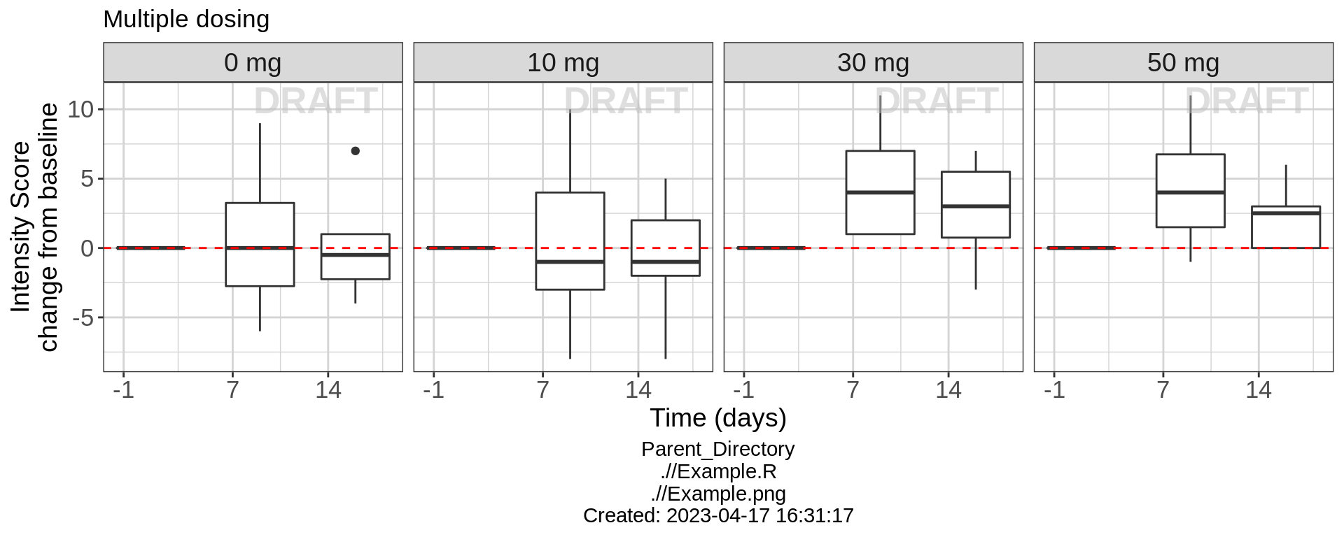
Dose Response
Intensity Score vs Dose
For this fast acting drug, an effect in change from baseline intensity score can actually be seen within the first 24 hours. In order to get an idea of the dose response relationship and make sure we are targeting an optimal dose, take a look at the response for a range of doses that were studied in the single ascending dose study. Plotting boxplots of the change from baseline intensity score against dose, you can see that starting at 10 mg, drug ABC123 has a clear effect on intensity score.
gg <- ggplot(pd_single_dosing %>% subset(NOMTIME == 24),
                aes(y = CHG, x = factor(DOSE)))
gg <- gg + geom_boxplot(aes(group = factor(DOSE)))
gg <- gg + ggtitle("Single dosing")
gg <- gg + geom_hline(yintercept = 0,
             color = "red",linetype = "dashed")
gg <- gg + theme(axis.text  = element_text(size = 13),
                 axis.title = element_text(size = 14),
                 strip.text = element_text(size = 14))
gg <- gg + ylab(paste0(pd_label,"\nchange from baseline"))
gg <- gg + xlab(dose_label)
gg <- gg + facet_wrap(~NOMTIME_label, nrow = 1)
gg <- gg + xgx_annotate_status()
gg <- gg + xgx_annotate_filenames(dirs)

gg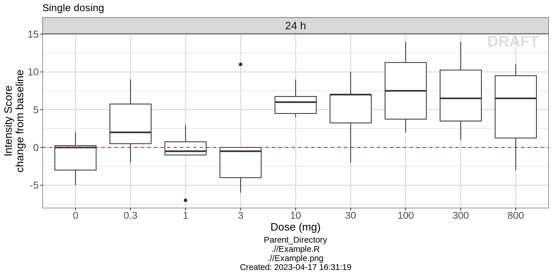
In the plot above, the doses are uniformly spaced, not proportionally spaced according to the numerical value of the doses. Producing this type of plot allows to clearly determine distinctions between different dose groups. However, it is wise to produce plots of dose vs response with dose on a scale proportional to the numerical value of the doses. This allows to more clearly see the shape of the dose-response relationship. Drug ABC123 has a nice dose-response curve shape that resembles a typical Emax model, appearing to plateau around 7.5 change from baseline in intensity score.
gg <- ggplot(pd_single_dosing %>% subset(NOMTIME == 24,),
               aes(y = CHG, x = DOSE, group = NOMTIME))
gg <- gg + xgx_stat_ci(conf_level = 0.975,
                       geom = c("point", "errorbar"),
                       alpha = 0.5)
gg <- gg + geom_hline(yintercept = 0, color = "red", linetype = "dashed")
gg <- gg + theme(axis.text  = element_text(size = 13),
                  axis.title = element_text(size = 14),
                  strip.text = element_text(size = 14))
gg <- gg + ggtitle("Single dosing")
gg <- gg + ylab(paste0(pd_label,"\nchange from baseline"))
gg <- gg + xlab(dose_label)
gg <- gg + facet_wrap(~NOMTIME_label, nrow = 1)
gg <- gg + xgx_annotate_status()
gg <- gg + xgx_annotate_filenames(dirs)

gg 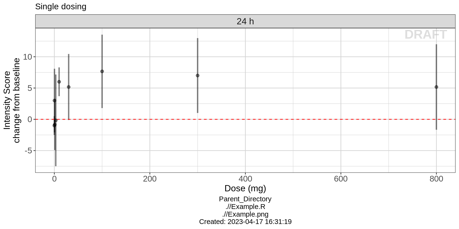
R Session Info
sessionInfo()## R version 4.1.0 (2021-05-18)
## Platform: x86_64-pc-linux-gnu (64-bit)
## Running under: Red Hat Enterprise Linux Server 7.9 (Maipo)
##
## Matrix products: default
## BLAS/LAPACK: /CHBS/apps/EB/software/imkl/2019.1.144-gompi-2019a/compilers_and_libraries_2019.1.144/linux/mkl/lib/intel64_lin/libmkl_gf_lp64.so
##
## locale:
## [1] LC_CTYPE=en_US.UTF-8 LC_NUMERIC=C LC_TIME=en_US.UTF-8 LC_COLLATE=en_US.UTF-8 LC_MONETARY=en_US.UTF-8
## [6] LC_MESSAGES=en_US.UTF-8 LC_PAPER=en_US.UTF-8 LC_NAME=C LC_ADDRESS=C LC_TELEPHONE=C
## [11] LC_MEASUREMENT=en_US.UTF-8 LC_IDENTIFICATION=C
##
## attached base packages:
## [1] stats graphics grDevices utils datasets methods base
##
## other attached packages:
## [1] caTools_1.18.2 DT_0.26 forcats_0.5.2 stringr_1.4.1 purrr_0.3.5 readr_2.1.3 tibble_3.1.8 tidyverse_1.3.2 xgxr_1.1.1
## [10] zoo_1.8-11 gridExtra_2.3 tidyr_1.2.1 dplyr_1.0.10 ggplot2_3.3.6
##
## loaded via a namespace (and not attached):
## [1] googledrive_2.0.0 colorspace_2.0-3 deldir_1.0-6 ellipsis_0.3.2 class_7.3-19 htmlTable_2.2.1 markdown_1.2
## [8] base64enc_0.1-3 fs_1.5.2 gld_2.6.2 rstudioapi_0.14 proxy_0.4-26 farver_2.1.1 Deriv_4.1.3
## [15] fansi_1.0.3 mvtnorm_1.1-3 lubridate_1.8.0 xml2_1.3.3 codetools_0.2-18 splines_4.1.0 cachem_1.0.6
## [22] rootSolve_1.8.2.2 knitr_1.40 Formula_1.2-4 jsonlite_1.8.3 broom_1.0.1 binom_1.1-1 cluster_2.1.3
## [29] dbplyr_2.2.1 png_0.1-7 compiler_4.1.0 httr_1.4.4 backports_1.4.1 assertthat_0.2.1 Matrix_1.5-1
## [36] fastmap_1.1.0 gargle_1.2.1 cli_3.4.1 prettyunits_1.1.1 htmltools_0.5.3 tools_4.1.0 gtable_0.3.1
## [43] glue_1.6.2 lmom_2.8 Rcpp_1.0.9 cellranger_1.1.0 jquerylib_0.1.4 vctrs_0.5.0 nlme_3.1-160
## [50] crosstalk_1.2.0 xfun_0.34 rvest_1.0.3 lifecycle_1.0.3 googlesheets4_1.0.1 MASS_7.3-58.1 scales_1.2.1
## [57] hms_1.1.2 expm_0.999-6 RColorBrewer_1.1-3 yaml_2.3.6 Exact_2.1 pander_0.6.4 sass_0.4.2
## [64] rpart_4.1.16 reshape_0.8.8 latticeExtra_0.6-30 stringi_1.7.8 highr_0.9 e1071_1.7-8 checkmate_2.1.0
## [71] boot_1.3-28 rlang_1.0.6 pkgconfig_2.0.3 bitops_1.0-7 evaluate_0.17 lattice_0.20-45 htmlwidgets_1.5.4
## [78] labeling_0.4.2 tidyselect_1.2.0 GGally_2.1.2 plyr_1.8.7 magrittr_2.0.3 R6_2.5.1 DescTools_0.99.42
## [85] generics_0.1.3 Hmisc_4.7-0 DBI_1.1.3 pillar_1.8.1 haven_2.5.1 foreign_0.8-82 withr_2.5.0
## [92] mgcv_1.8-41 survival_3.4-0 RCurl_1.98-1.4 nnet_7.3-17 crayon_1.5.2 modelr_0.1.9 interp_1.1-2
## [99] utf8_1.2.2 tzdb_0.3.0 rmarkdown_2.17 progress_1.2.2 jpeg_0.1-9 grid_4.1.0 readxl_1.4.1
## [106] minpack.lm_1.2-1 data.table_1.14.2 reprex_2.0.2 digest_0.6.30 munsell_0.5.0 bslib_0.4.0