Survival Regression with Time-Varying Covariates

In this notebook, we use TorchSurv to train a model that predicts relative risk given time-varying covariates. We use the heart data set from the survival package in R. After training the model, we evaluate the predictive performance using evaluation metrics implemented in TorchSurv.

The dataset contains survival of patients on the waiting list for the Stanford heart transplant program for 103 patients.

1. Dependencies

To run this notebook, dependencies must be installed. the recommended method is to use our development conda environment (preferred). Instruction can be found here to install all optional dependencies. The other method is to install only required packages using the command line below:

# Install only required packages (optional)
# %pip install matplotlib
# %pip install sklearn
# %pip install pandas

import warnings

warnings.filterwarnings("ignore")

import pandas as pd
import torch
import torch.nn as nn

# PyTorch boilerplate - see https://github.com/Novartis/torchsurv/blob/main/docs/notebooks/helpers_introduction.py
from helpers_time_varying import GroupedDataset, collate_fn, expand_log_hz, expand_log_hz_survival, plot_losses
from sklearn.model_selection import train_test_split
from torch.utils.data import DataLoader

# Our package
from torchsurv.loss import cox, survival
from torchsurv.metrics.auc import Auc
from torchsurv.metrics.brier_score import BrierScore
from torchsurv.metrics.cindex import ConcordanceIndex

# Set seed
seed = 15
torch.manual_seed(seed)
torch.cuda.manual_seed(seed)
torch.cuda.manual_seed_all(seed)

# Issue with eager mode
# torch._dynamo.config.suppress_errors = True  # Suppress inductor errors
# torch._dynamo.reset()  # Reset the backend

# Constant parameters across models
BATCH_SIZE = 32  # batch size = number of patients
EPOCHS = 100  # maximum number of epochs
LEARNING_RATE = 1e-2  # learning rate

2. Dataset

In datasets with time-varying covariates, each individual may contribute multiple rows of observations. This occurs because a patient can be measured repeatedly over time, with covariates updated at each measurement interval. The variables start and stop denote the time interval during which the covariates in a given row are valid, and within which the event indicator corresponds to the occurrence (or non-occurrence) of an event.

# Load heart dataset from R survival
df = pd.read_csv("heart.csv")
df.head(5)

# number of samples
print(f"Number of samples: {df.shape[0]}")

Number of samples: 172

The dataset contains the features:

• age: age - 48 years

• year: year of acceptance (in years after 1 Nov 1967)

• surgery: prior bypass surgery 1=yes

• transplant: received transplant 1=yes

• id: patient id

Additionally, it contains our survival targets:

• start, stop, event: Entry time, exit time and status for this interval of time.

Further, we add two columns: time for the latest observation time and event_at_time for the event status at that time. These variables remain constant across all rows corresponding to the same patient.

# Add time column (max stop per id)
df["time"] = df.groupby("id")["stop"].transform("max")

# Add column for event at that time
df["event_at_time"] = df.apply(
    lambda row: df[(df["id"] == row["id"]) & (df["stop"] == row["time"])]["event"].iloc[0],
    axis=1,
)

df.head(5)

	start	stop	event	age	year	surgery	transplant	id	time	event_at_time
0	0.0	50.0	1	-17.155373	0.123203	0	0	1	50.0	1
1	0.0	6.0	1	3.835729	0.254620	0	0	2	6.0	1
2	0.0	1.0	0	6.297057	0.265572	0	0	3	16.0	1
3	1.0	16.0	1	6.297057	0.265572	0	1	3	16.0	1
4	0.0	36.0	0	-7.737166	0.490075	0	0	4	39.0	1

Next, we set up the data loaders for training, validation, and testing. Here, the BATCH_SIZE corresponds to the number of patient IDs per batch. We cannot sample a fixed number of rows at random as in the non time-varying covariates setting, because for each selected patient ID we must include all rows associated with that individual.

# Split by IDs
ids = df["id"].unique()

train_ids, test_ids = train_test_split(ids, test_size=0.3, random_state=42)
train_ids, val_ids = train_test_split(train_ids, test_size=0.3, random_state=42)

df_train = df[df.id.isin(train_ids)]
df_val = df[df.id.isin(val_ids)]
df_test = df[df.id.isin(test_ids)]

train_dataset = GroupedDataset(df_train)
val_dataset = GroupedDataset(df_val)
test_dataset = GroupedDataset(df_test)

dataloader_train = DataLoader(train_dataset, batch_size=BATCH_SIZE, shuffle=True, collate_fn=collate_fn)

dataloader_val = DataLoader(
    val_dataset,
    batch_size=len(val_dataset),  # full batch
    shuffle=False,
    collate_fn=collate_fn,
)

dataloader_test = DataLoader(test_dataset, batch_size=len(test_dataset), shuffle=False, collate_fn=collate_fn)

Let \(m\) be the total number of rows in the batch (the total number of observations across all individuals), and let \(n\) be the number of unique IDs (where \(n\) = BATCH_SIZE), with \(m \geq n\). Further let \(p\) denote the number of covariates.

The dataloader returns five outputs: - x: a feature matrix of shape = (m, p) - event, time: event indicator and event time, each of shape (n,) - id, start: index vector of shape = (m,)

For each observation index \(k\) (where \(0\leq k\leq m\)), the feature vector for individual id[k] at the observation time indicated by start[k] is x[k,:]. In plain language: id tells you which individual, start tells you which time index for that individual.

# Sanity check
x, (event, time), id, start = next(iter(dataloader_train))
num_features = x.size(1)

print(f"x (shape)    = {x.shape}")
print(f"num_features = {num_features}")
print(f"event        = {event.shape}")
print(f"time         = {time.shape}")
print(f"id           = {id.shape}")
print(f"start        = {start.shape}")

x (shape)    = torch.Size([54, 4])
num_features = 4
event        = torch.Size([32, 1])
time         = torch.Size([32, 1])
id           = torch.Size([54])
start        = torch.Size([54])

3. Cox Model

In this section, we use the Extended Cox proportional hazards model. Given covariates \(x_{i}(t)\), a vector of size \(p\), the hazard of patient \(i\) has the form

\[h_i(t) =\lambda_{0}(t)\: \lambda_i(t)\]

The baseline hazard \(\lambda_{0}(t)\) is identical across subjects (i.e., has no dependency on \(i\)). The subject-specific risk of event occurrence is captured through the relative hazards \(\{\lambda_i(t)\}_{i = 1, \dots, N}\).

In the traditional Cox proportional hazards model, the log-relative hazard is modeled as a linear combination of covariates:

\[\log \lambda_i(t) = x_i(t)^\top \beta.\]

In contrast, we allow the log-relative hazard \(\log \lambda_i(t)\) to be modeled using a neural network. A key assumption in the Extended Cox model is that the model parameters are not time-varying. Consequently, we define a neural network such that

\[\log \lambda_i(t) = f_\theta(x_i(t)),\]

where \(\theta\) represents the parameters of the neural network – which are constant over time.

For instance, we can train a multi-layer perceptron (MLP) to model the log-relative hazard \(\log \lambda_i(t)\).

3.1. MLP model for log relative hazards

# Initiate Extended Cox model
cox_model = torch.nn.Sequential(
    torch.nn.BatchNorm1d(num_features),  # Batch normalization
    torch.nn.Linear(num_features, 16),
    torch.nn.ReLU(),
    torch.nn.Dropout(),
    torch.nn.Linear(16, 64),
    torch.nn.ReLU(),
    torch.nn.Dropout(),
    torch.nn.Linear(64, 32),
    torch.nn.ReLU(),
    torch.nn.Dropout(),
    torch.nn.Linear(32, 1),  # Estimating log hazards for Cox models
)

3.2. Model training

The function cox.neg_partial_log_likelihood in the time-varying covariate setting expects the matrix \(\log \lambda_i(t)\) evaluated for id (by rows) and for time \(t\) (by columns), resulting in an \((n, n)\) matrix.

When we pass x through our neural network, we obtain log_hz_short which produces a vector of shape \((m,)\). Each entry log_hz_short[k] corresponds to the value \(\log \lambda_i(t) = f_\theta(x_i(t))\) for the individual \(i =\)id[k] at the time interval beginning at \(t =\) start[k].

To convert this vector into the required \((n, n)\) matrix format, we use the helper function expand_log_hz, which reformats the model output into the log_hz matrix expected by the loss function.

torch.manual_seed(42)

# Init optimizer for Cox
optimizer = torch.optim.RMSprop(cox_model.parameters(), lr=LEARNING_RATE)

# Initiate empty list to store the loss on the train and validation sets
train_losses = []
val_losses = []

# training loop
for epoch in range(EPOCHS):
    epoch_loss = torch.tensor(0.0)
    for _, batch in enumerate(dataloader_train):
        x, (event, time), id, start = batch

        optimizer.zero_grad()
        log_hz_short = cox_model(x)  # shape = (m,)

        # expand log_hz to row = id, column = time
        log_hz = expand_log_hz(id, start, time, log_hz_short)  # shape  = (n,n)

        loss = cox.neg_partial_log_likelihood(log_hz, event, time, reduction="mean")
        loss.backward()
        optimizer.step()
        epoch_loss += loss.detach()

    if epoch % (EPOCHS // 10) == 0:
        print(f"Epoch: {epoch:03}, Training loss: {epoch_loss:0.2f}")

    # Record loss on train and test sets
    train_losses.append(epoch_loss)
    with torch.no_grad():
        x, (event, time), id, start = batch = next(iter(dataloader_val))
        val_losses.append(
            cox.neg_partial_log_likelihood(
                expand_log_hz(id, start, time, cox_model(x)),
                event,
                time,
                reduction="mean",
            )
        )

Epoch: 000, Training loss: 5.39
Epoch: 010, Training loss: 5.56
Epoch: 020, Training loss: 5.42
Epoch: 030, Training loss: 4.92
Epoch: 040, Training loss: 4.86
Epoch: 050, Training loss: 5.22
Epoch: 060, Training loss: 4.68
Epoch: 070, Training loss: 4.86
Epoch: 080, Training loss: 5.15
Epoch: 090, Training loss: 4.92

We can visualize the training and validation losses.

plot_losses(train_losses, val_losses, "Cox")

3.3. Evaluation metrics

We evaluate the predictive performance of the model using

• the concordance index (C-index), which measures the probability that a model correctly predicts which of two comparable samples will experience an event first based on their estimated risk scores,

• the Area Under the Receiver Operating Characteristic Curve (AUC), which measures the probability that a model correctly predicts which of two comparable samples will experience an event by time t based on their estimated risk scores.

• the Brier score, which measures the model’s calibration by calculating the mean square error between the estimated survival function and the empirical (i.e., in-sample) event status.

For the Cox model, to estimate the survival function on the test set, we first need to estimate the baseline survival function on the training set:

cox_model.eval()
with torch.no_grad():
    x, (event, time), id, start = next(iter(dataloader_train))
    log_hz = expand_log_hz(id, start, time, cox_model(x))  # log hazard on train set
    baseline_surv = cox.baseline_survival_function(log_hz, event, time)  # baseline survival function

We then evaluate the subject-specific relative hazards and on the survival function on the test set.

with torch.no_grad():
    # test event and test time of length n
    test_x, (test_event, test_time), test_id, test_start = next(iter(dataloader_test))
    test_log_hz = expand_log_hz(test_id, test_start, test_time, cox_model(test_x))  # log hazard of test set

# Compute the survival probability
test_surv = cox.survival_function_cox(baseline_surv, test_log_hz, test_time)  # shape = (n,n)

We obtain the concordance index, and its confidence interval

# Concordance index
cox_cindex = ConcordanceIndex()
print("Cox model performance:")
print(f"Concordance-index   = {cox_cindex(test_log_hz, test_event, test_time)}")
print(f"Confidence interval = {cox_cindex.confidence_interval()}")

Cox model performance:
Concordance-index   = 0.5808457732200623
Confidence interval = tensor([0.3468, 0.8149])

We can also test whether the observed concordance index is greater than 0.5. The statistical test is specified with H0: c-index = 0.5 and Ha: c-index > 0.5. The p-value of the statistical test is

# H0: cindex = 0.5, Ha: cindex > 0.5
print("p-value = {}".format(cox_cindex.p_value(alternative="greater")))

p-value = 0.24920672178268433

For time-dependent prediction (e.g., 5-year mortality), the C-index is not a proper measure. Instead, it is recommended to use the AUC. The probability to correctly predicts which of two comparable patients will experience an event by 5-year based on their estimated risk scores is the AUC evaluated at 5-year (1825 days) obtained with

cox_auc = Auc()

new_time = torch.tensor(1095.0)
log_hz_t = expand_log_hz(test_id, test_start, new_time.unsqueeze(0), cox_model(test_x))

# auc evaluated at new time = 1095, 3 year
print(f"AUC 3-yr             = {cox_auc(log_hz_t, test_event, test_time, new_time=new_time)}")
print(f"AUC 3-yr (conf int.) = {cox_auc.confidence_interval()}")

AUC 3-yr             = tensor([0.6061])
AUC 3-yr (conf int.) = tensor([0.4005, 0.8117])

As before, we can test whether the observed Auc at 3-year is greater than 0.5. The statistical test is specified with H0: auc = 0.5 and Ha: auc > 0.5. The p-value of the statistical test is

print(f"AUC (p_value) = {cox_auc.p_value(alternative='greater')}")

AUC (p_value) = tensor([0.1560])

Lastly, we can evaluate the time-dependent Brier score and the integrated Brier score

cox_brier_score = BrierScore()

# brier score at last 5 times
print(f"Brier score             = {cox_brier_score(test_surv, test_event, test_time)[-5:]}")
print(f"Brier score (conf int.) = {cox_brier_score.confidence_interval()[:, -5:]}")

# integrated brier score
print(f"Integrated Brier score  = {cox_brier_score.integral()}")

Brier score             = tensor([0.1632, 0.1306, 0.0947, 0.0484, 0.0199])
Brier score (conf int.) = tensor([[0.1053, 0.0692, 0.0320, 0.0000, 0.0033],
        [0.2211, 0.1920, 0.1573, 0.1055, 0.0364]])
Integrated Brier score  = 0.16062888503074646

We can test whether the time-dependent Brier score is smaller than what would be expected if the survival model was not providing accurate predictions beyond random chance. We use a bootstrap permutation test and obtain the p-value with:

# H0: bs = bs0, Ha: bs < bs0;
# where bs0 is the expected brier score if the survival model was not providing accurate predictions beyond random chance.

# p-value for brier score at last 5 times
print(f"Brier score (p-val) = {cox_brier_score.p_value(alternative='less')[-5:]}")

Brier score (p-val) = tensor([0.5650, 0.5510, 0.5550, 0.5270, 0.3940])

4. Flexible Survival Model

In this section, we use the Flexible Survival model. Given covariates \(x_{i}(t)\), a vector of size \(p\), the log hazard of patient \(i\) at time \(t\) is the output a neural network:

\[\log h_i (t) = f_{\theta}(x_{i}(t), t)\]

where \(\theta\) denotes the parameters of the neural network (which may depend on time). For instance, we can train a multi-layer perceptron (MLP) to model the log hazard \(\log h_i(t)\).

4.1. MLP model for log hazard

# Same architecture than Cox model, beside inputs dimension
class SurvivalModel(nn.Module):
    def __init__(self, num_features):
        super().__init__()
        self.net = nn.Sequential(
            nn.Linear(num_features + 1, 32),
            nn.ReLU(),
            nn.Dropout(0.1),
            nn.Linear(32, 64),
            nn.ReLU(),
            nn.Dropout(0.1),
            nn.Linear(64, 1),  # output log-hazard for this x,t
        )

    def forward(self, x, t):
        # x: [N, F], t: [T, 1]
        N, F = x.shape
        T = t.shape[0]

        # Expand x to [N, T, F]
        x_exp = x.unsqueeze(1).expand(N, T, F)
        # Expand t to [N, T, 1]
        t_exp = t.unsqueeze(0).expand(N, T, 1)
        # Concatenate along feature dim
        xt = torch.cat([x_exp, t_exp], dim=2)  # [N, T, F+1]

        # Flatten first two dims for processing
        xt_flat = xt.reshape(N * T, F + 1)
        out_flat = self.net(xt_flat)  # [N*T, 1]

        # Reshape back to [N, T]
        out = out_flat.reshape(N, T)
        return out


# instantiate
survival_model = SurvivalModel(num_features)

4.2. Model training

The Flexible Survival Model relies on a numerical approximation of the cumulative hazard in order to compute the likelihood. As a result, the log-hazard must be evaluated over a set of time points specified in eval_time. In practice, these evaluation times should be as uniformly distributed as possible, and they must include all observed event or censoring times stored in time. Further, we denote by \(u\) the number of evaluation times.

Below is the code used to construct the evaluation grid:

# Eval time at which to evaluate the hazard
dt = 10.0
time_train = torch.tensor(df_train["time"].values, device=time.device, dtype=torch.float)
eval_time = torch.arange(0, time_train.max() + dt, dt)
extra_times = time_train.squeeze()[~torch.isin(time_train.squeeze(), eval_time)]
eval_time = torch.cat([eval_time, extra_times])  # Add original time points
eval_time = torch.unique(eval_time)  # sort and remove duplicate
eval_time = eval_time.unsqueeze(1)

The function survival.neg_log_likelihood for time-varying covariates expects a matrix \(\log h_i(t)\) evaluated for id (rows) and for all eval_time (columns). This yields an \((n, u)\) matrix, where \(u = |\)eval_time\(|\).

When we pass x and eval_time through our survival_model, we obtain log_hz_long, which returns a matrix of shape \((m, u)\). Each entry log_hz_long[k, l] corresponds to the value \(\log h_i(t) = f_\theta(x_i(t), t)\) for the individual \(i =\)id[k] at the time \(t =\) eval_time[l].

where

- id[k] identifies the individual \(i\),

- start[k] marks the beginning of the time interval for which the covariates \(x_i(t)\) are valid, and

- eval_time[l] is the evaluation time at which the hazard is computed.

To transform this \((m, u)\) output into the required \((n, u)\) format, we use the helper function expand_log_hz_survival, which aggregates the per-row outputs into the full log_hz matrix expected by the loss function.

torch.manual_seed(42)

# Init optimizer for Weibull
optimizer = torch.optim.Adam(survival_model.parameters(), lr=LEARNING_RATE)

# Initialize empty list to store loss on train and validation sets
train_losses = []
val_losses = []

# training loop
for epoch in range(EPOCHS):
    epoch_loss = torch.tensor(0.0)
    for _, batch in enumerate(dataloader_train):
        x, (event, time), id, start = batch
        optimizer.zero_grad()
        log_hz_long = survival_model(x, eval_time)  # shape = (m,u)

        # expand log_hz to row = id, column = time
        log_hz = expand_log_hz_survival(id, start, eval_time, log_hz_long)  # shape = (n,u)

        loss = survival.neg_log_likelihood(log_hz, event, time, reduction="mean", eval_time=eval_time)
        loss.backward()
        optimizer.step()
        epoch_loss += loss.detach()

    if epoch % (EPOCHS // 10) == 0:
        print(f"Epoch: {epoch:03}, Training loss: {epoch_loss:0.2f}")

    # Record losses for the following figure
    train_losses.append(epoch_loss)
    with torch.no_grad():
        x, (event, time), id, start = next(iter(dataloader_val))
        val_losses.append(
            survival.neg_log_likelihood(
                expand_log_hz_survival(id, start, eval_time, survival_model(x, eval_time)),
                event,
                time,
                eval_time=eval_time,
                reduction="mean",
            )
        )

Epoch: 000, Training loss: 1397500800.00
Epoch: 010, Training loss: 211.00
Epoch: 020, Training loss: 266.84
Epoch: 030, Training loss: 208.24
Epoch: 040, Training loss: 218.81
Epoch: 050, Training loss: 237.73
Epoch: 060, Training loss: 235.83
Epoch: 070, Training loss: 268.04
Epoch: 080, Training loss: 193.11
Epoch: 090, Training loss: 216.74

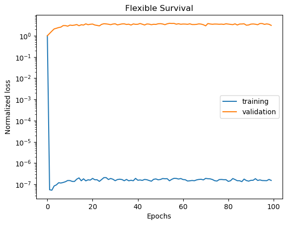
We can visualize the training and validation losses.

plot_losses(train_losses, val_losses, "Flexible Survival")

4.3. Evaluation Metrics

As for the Extended Cox Model, we evaluate the predictive performance of the model using the C-index, the AUC and the Brier score.

We begin by computing the subject-specific log-hazard at every time \(t\) recorded in time for the test set (test_log_hz), as well as the log-hazard evaluated at all times in eval_time (test_log_hz_eval_time).

with torch.no_grad():
    # test event and test time of length n
    test_x, (test_event, test_time), test_id, test_start = next(iter(dataloader_test))
    log_hz_eval_time_long = survival_model(test_x, eval_time)
    test_log_hz_eval_time = expand_log_hz_survival(
        test_id, test_start, eval_time, log_hz_eval_time_long
    )  # shape = (n, u)
    test_log_hz = expand_log_hz_survival(test_id, test_start, test_time, log_hz_eval_time_long)  # shape = (n, n)

We then obtain the subject-specific survival at every time \(t\) recorded in time:

test_surv = survival.survival_function(test_log_hz_eval_time, test_time, eval_time)  # shape = (n,n)

We can evaluate the concordance index, its confidence interval and the p-value of the statistical test testing whether the c-index is greater than 0.5:

# Concordance index
survival_cindex = ConcordanceIndex()
print("Cox model performance:")
print(f"Concordance-index   = {survival_cindex(test_log_hz, test_event, test_time)}")
print(f"Confidence interval = {survival_cindex.confidence_interval()}")

# H0: cindex = 0.5, Ha: cindex > 0.5
print("p-value = {}".format(survival_cindex.p_value(alternative="greater")))

Cox model performance:
Concordance-index   = 0.5
Confidence interval = tensor([0.2264, 0.7736])
p-value = 0.5

For time-dependent prediction (e.g., 3-year mortality), the C-index is not a proper measure. Instead, it is recommended to use the AUC. The probability to correctly predicts which of two comparable patients will experience an event by 5-year based on their estimated risk scores is the AUC evaluated at 3-year (1095 days) obtained with

survival_auc = Auc()

new_time = torch.tensor(1095.0)

# subject-specific log hazard at 3-yr
log_hz_t = expand_log_hz_survival(test_id, test_start, new_time.unsqueeze(0), log_hz_eval_time_long)

# auc evaluated at new time = 1095, 3 year
print(f"AUC 3-yr             = {survival_auc(log_hz_t, test_event, test_time, new_time=new_time)}")
print(f"AUC 3-yr (conf int.) = {survival_auc.confidence_interval()}")

print(f"AUC (p_value) = {survival_auc.p_value(alternative='greater')}")

AUC 3-yr             = tensor([0.1061])
AUC 3-yr (conf int.) = tensor([0.0396, 0.1725])
AUC (p_value) = tensor([1.])

Lastly, we can evaluate the time-dependent Brier score and the integrated Brier score

survival_brier_score = BrierScore()

# brier score at last 5 times
print(f"Brier score             = {survival_brier_score(test_surv, test_event, test_time)[-5:]}")
print(f"Brier score (conf int.) = {survival_brier_score.confidence_interval()[:, -5:]}")

# integrated brier score
print(f"Integrated Brier score  = {survival_brier_score.integral()}")

# H0: bs = bs0, Ha: bs < bs0;
# where bs0 is the expected brier score if the survival model was not providing accurate predictions beyond random chance.

# p-value for brier score at last 5 times
print(f"Brier score (p-val)        = {survival_brier_score.p_value(alternative='less')[-5:]}")

Brier score             = tensor([0.6305, 0.6558, 0.6556, 0.6546, 0.6546])
Brier score (conf int.) = tensor([[0.4710, 0.5012, 0.5009, 0.4994, 0.4994],
        [0.7901, 0.8104, 0.8104, 0.8099, 0.8099]])
Integrated Brier score  = 0.6031082272529602
Brier score (p-val)        = tensor([0.5450, 0.4160, 0.4130, 0.3910, 0.3930])

5. Models comparison

We can compare the predictive performance of the Cox proportional hazards model against the Flexible Survival model.

Comparing the Concordance index

The statistical test is formulated as follows, H0: cindex cox = cindex flexible survival, Ha: cindex cox > cindex flexible survival

print(f"Cox cindex     = {cox_cindex.cindex}")
print(f"Flexible Survival cindex = {survival_cindex.cindex}")
print(f"p-value        = {cox_cindex.compare(survival_cindex)}")

Cox cindex     = 0.5808457732200623
Flexible Survival cindex = 0.5
p-value        = 0.3301258087158203

Comparing the AUC at 3-year

The statistical test is formulated as follows, H0: 3-yr auc cox = 3-yr auc flexible survival, Ha: 5-yr auc cox > 5-yr auc flexible survival

print(f"Cox 5-yr AUC     = {cox_auc.auc}")
print(f"Flexible Survival 5-yr AUC = {survival_auc.auc}")
print(f"p-value          = {cox_auc.compare(survival_auc)}")

Cox 5-yr AUC     = tensor([0.6061])
Flexible Survival 5-yr AUC = tensor([0.1061])
p-value          = tensor([6.1089e-05])

Comparing the Brier-Score at 3-year

The statistical test is formulated as follows, H0: 3-yr bs cox = 3-yr bs flexible survival, Ha: 3-yr bs cox > 3-yr bs flexible survival

print(f"Cox 3-yr BS     = {cox_brier_score.brier_score[16]}")
print(f"Flexible Survival 3-yr BS = {survival_brier_score.brier_score[16]}")
print(f"p-value          = {cox_brier_score.compare(survival_brier_score)[16]}")

Cox 3-yr BS     = 0.25146567821502686
Flexible Survival 3-yr BS = 0.5034263730049133
p-value          = 0.002828118624165654