Survival Regression#
In this notebook, we use TorchSurv to train a model that predicts relative risk of breast cancer recurrence. We use a public data set, the German Breast Cancer Study Group 2 (GBSG2). After training the model, we evaluate the predictive performance using evaluation metrics implemented in TorchSurv.
We first load the dataset using the package lifelines. The GBSG2 dataset contains features and recurrence free survival time (in days) for 686 women undergoing hormonal treatment.
1. Dependencies#
To run this notebook, dependencies must be installed. the recommended method is to use our development conda environment (preferred). Instruction can be found here to install all optional dependencies. The other method is to install only required packages using the command line below:
[1]:
# Install only required packages (optional)
# %pip install lifelines
# %pip install matplotlib
# %pip install sklearn
# %pip install pandas
[2]:
import warnings

warnings.filterwarnings("ignore")
[3]:
import lifelines
import pandas as pd
import torch

# PyTorch boilerplate - see https://github.com/Novartis/torchsurv/blob/main/docs/notebooks/helpers_introduction.py
from helpers_introduction import Custom_dataset, plot_losses
from sklearn.model_selection import train_test_split
from torch.utils.data import DataLoader

# Our package
from torchsurv.loss import cox, weibull
from torchsurv.metrics.auc import Auc
from torchsurv.metrics.brier_score import BrierScore
from torchsurv.metrics.cindex import ConcordanceIndex
[4]:
# Issue with eager mode
# torch._dynamo.config.suppress_errors = True  # Suppress inductor errors
# torch._dynamo.reset()  # Reset the backend
[5]:
# Constant parameters across models
# Detect available accelerator; Downgrade batch size if only CPU available
if any([torch.cuda.is_available(), torch.backends.mps.is_available()]):
    print("CUDA-enabled GPU/TPU is available.")
    BATCH_SIZE = 128  # batch size for training
else:
    print("No CUDA-enabled GPU found, using CPU.")
    BATCH_SIZE = 32  # batch size for training

EPOCHS = 100
LEARNING_RATE = 1e-2
CUDA-enabled GPU/TPU is available.
2. Dataset#
[6]:
# Load GBSG2 dataset
df = lifelines.datasets.load_gbsg2()
df.head(5)
[6]:
| horTh | age | menostat | tsize | tgrade | pnodes | progrec | estrec | time | cens | |
|---|---|---|---|---|---|---|---|---|---|---|
| 0 | no | 70 | Post | 21 | II | 3 | 48 | 66 | 1814 | 1 |
| 1 | yes | 56 | Post | 12 | II | 7 | 61 | 77 | 2018 | 1 |
| 2 | yes | 58 | Post | 35 | II | 9 | 52 | 271 | 712 | 1 |
| 3 | yes | 59 | Post | 17 | II | 4 | 60 | 29 | 1807 | 1 |
| 4 | no | 73 | Post | 35 | II | 1 | 26 | 65 | 772 | 1 |
The dataset contains the features:
horTh: hormonal therapy, a factor at two levels (yes and no).age: age of the patients in years.menostat: menopausal status, a factor at two levels pre (premenopausal) and post (postmenopausal).tsize: tumor size (in mm).tgrade: tumor grade, a ordered factor at levels I < II < III.pnodes: number of positive nodes.progrec: progesterone receptor (in fmol).estrec: estrogen receptor (in fmol).
Additionally, it contains our survival targets:
time: recurrence free survival time (in days).cens: event indicator (0- censored, 1- event).
One common approach is to use a one hot encoder to convert them into numerical features. We then separate the dataframes into features X and labels y. The following code also partitions the labels and features into training and testing cohorts.
Data preparation:
[7]:
df_onehot = pd.get_dummies(df, columns=["horTh", "menostat", "tgrade"]).astype("float")
df_onehot.drop(
    ["horTh_no", "menostat_Post", "tgrade_I"],
    axis=1,
    inplace=True,
)
df_onehot.head(5)
[7]:
| age | tsize | pnodes | progrec | estrec | time | cens | horTh_yes | menostat_Pre | tgrade_II | tgrade_III | |
|---|---|---|---|---|---|---|---|---|---|---|---|
| 0 | 70.0 | 21.0 | 3.0 | 48.0 | 66.0 | 1814.0 | 1.0 | 0.0 | 0.0 | 1.0 | 0.0 |
| 1 | 56.0 | 12.0 | 7.0 | 61.0 | 77.0 | 2018.0 | 1.0 | 1.0 | 0.0 | 1.0 | 0.0 |
| 2 | 58.0 | 35.0 | 9.0 | 52.0 | 271.0 | 712.0 | 1.0 | 1.0 | 0.0 | 1.0 | 0.0 |
| 3 | 59.0 | 17.0 | 4.0 | 60.0 | 29.0 | 1807.0 | 1.0 | 1.0 | 0.0 | 1.0 | 0.0 |
| 4 | 73.0 | 35.0 | 1.0 | 26.0 | 65.0 | 772.0 | 1.0 | 0.0 | 0.0 | 1.0 | 0.0 |
[8]:
df_train, df_test = train_test_split(df_onehot, test_size=0.3)
df_train, df_val = train_test_split(df_train, test_size=0.3)
print(f"(Sample size) Training:{len(df_train)} | Validation:{len(df_val)} |Testing:{len(df_test)}")
(Sample size) Training:336 | Validation:144 |Testing:206
Let us setup the dataloaders for training, validation and testing.
[9]:
# Dataloader
dataloader_train = DataLoader(Custom_dataset(df_train), batch_size=BATCH_SIZE, shuffle=True)
dataloader_val = DataLoader(Custom_dataset(df_val), batch_size=len(df_val), shuffle=False)
dataloader_test = DataLoader(Custom_dataset(df_test), batch_size=len(df_test), shuffle=False)
[10]:
# Sanity check
x, (event, time) = next(iter(dataloader_train))
num_features = x.size(1)

print(f"x (shape)    = {x.shape}")
print(f"num_features = {num_features}")
print(f"event        = {event.shape}")
print(f"time         = {time.shape}")
x (shape)    = torch.Size([128, 9])
num_features = 9
event        = torch.Size([128])
time         = torch.Size([128])
3. Cox Model#
In this section, we use the Cox proportional hazards model. Given covariates \(x_{i}\), a vector of size \(p\), the hazard of patient \(i\) has the form
The baseline hazard \(\lambda_{0}(t)\) is identical across subjects (i.e., has no dependency on \(i\)). The subject-specific risk of event occurrence is captured through the relative hazards \(\{\lambda_i\}_{i = 1, \dots, N}\).
In the traditional Cox proportional hazards model, the log relative hazards are modeled as a linear combination of covariates: i.e., \(\log \lambda_i = x_{i}^T \beta\). In contrast, we allow the log relative hazards \(\log \lambda_i\) to be modeled by a neural network. For example, here we train a multi-layer perceptron (MLP) to model the log relative hazards \(\log\lambda_i\). Patients with lower recurrence time are assumed to have higher risk of event.
3.1. MLP model for log relative hazards#
[11]:
# Initiate Cox model
cox_model = torch.nn.Sequential(
    torch.nn.BatchNorm1d(num_features),  # Batch normalization
    torch.nn.Linear(num_features, 32),
    torch.nn.ReLU(),
    torch.nn.Dropout(),
    torch.nn.Linear(32, 64),
    torch.nn.ReLU(),
    torch.nn.Dropout(),
    torch.nn.Linear(64, 1),  # Estimating log hazards for Cox models
)
3.2. Model training#
[12]:
torch.manual_seed(42)

# Init optimizer for Cox
optimizer = torch.optim.Adam(cox_model.parameters(), lr=LEARNING_RATE)

# Initiate empty list to store the loss on the train and validation sets
train_losses = []
val_losses = []

# training loop
for epoch in range(EPOCHS):
    epoch_loss = torch.tensor(0.0)
    for _, batch in enumerate(dataloader_train):
        x, (event, time) = batch
        optimizer.zero_grad()
        log_hz = cox_model(x)  # shape = (16, 1)
        loss = cox.neg_partial_log_likelihood(log_hz, event, time, reduction="mean")
        loss.backward()
        optimizer.step()
        epoch_loss += loss.detach()

    if epoch % (EPOCHS // 10) == 0:
        print(f"Epoch: {epoch:03}, Training loss: {epoch_loss:0.2f}")

    # Record loss on train and test sets
    train_losses.append(epoch_loss)
    with torch.no_grad():
        x, (event, time) = next(iter(dataloader_val))
        val_losses.append(cox.neg_partial_log_likelihood(cox_model(x), event, time, reduction="mean"))
Epoch: 000, Training loss: 12.40
Epoch: 010, Training loss: 12.07
Epoch: 020, Training loss: 11.99
Epoch: 030, Training loss: 11.94
Epoch: 040, Training loss: 11.76
Epoch: 050, Training loss: 11.75
Epoch: 060, Training loss: 11.81
Epoch: 070, Training loss: 11.70
Epoch: 080, Training loss: 11.63
Epoch: 090, Training loss: 11.62
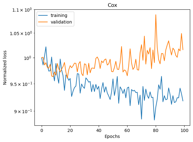
We can visualize the training and validation losses.
[13]:
plot_losses(train_losses, val_losses, "Cox")
3.3. Evaluation metrics#
We evaluate the predictive performance of the model using
the concordance index (C-index), which measures the probability that a model correctly predicts which of two comparable samples will experience an event first based on their estimated risk scores,
the Area Under the Receiver Operating Characteristic Curve (AUC), which measures the probability that a model correctly predicts which of two comparable samples will experience an event by time t based on their estimated risk scores.
the Brier score, which measures the model’s calibration by calculating the mean square error between the estimated survival function and the empirical (i.e., in-sample) event status.
For the Cox model, to estimate the survival function on the test set, we first need to estimate the baseline survival function on the training set:
[14]:
cox_model.eval()
with torch.no_grad():
    x, (event, time) = next(iter(dataloader_train))
    log_hz = cox_model(x)  # log hazard on train set
    baseline_surv = cox.baseline_survival_function(log_hz, event, time)  # baseline survival function
We then evaluate the subject-specific relative hazards and on the survival function on the test set
[15]:
with torch.no_grad():
    # test event and test time of length n
    test_x, (test_event, test_time) = next(iter(dataloader_test))
    test_log_hz = cox_model(test_x)  # log hazard of length n

# Compute the survival probability
test_surv = cox.survival_function_cox(baseline_surv, test_log_hz, test_time)  # shape = (n,n)
We obtain the concordance index, and its confidence interval
[16]:
# Concordance index
cox_cindex = ConcordanceIndex()
print("Cox model performance:")
print(f"Concordance-index   = {cox_cindex(test_log_hz, test_event, test_time)}")
print(f"Confidence interval = {cox_cindex.confidence_interval()}")
Cox model performance:
Concordance-index   = 0.6240726709365845
Confidence interval = tensor([0.5151, 0.7331])
We can also test whether the observed concordance index is greater than 0.5. The statistical test is specified with H0: c-index = 0.5 and Ha: c-index > 0.5. The p-value of the statistical test is
[17]:
# H0: cindex = 0.5, Ha: cindex > 0.5
print("p-value = {}".format(cox_cindex.p_value(alternative="greater")))
p-value = 0.012831330299377441
For time-dependent prediction (e.g., 5-year mortality), the C-index is not a proper measure. Instead, it is recommended to use the AUC. The probability to correctly predicts which of two comparable patients will experience an event by 5-year based on their estimated risk scores is the AUC evaluated at 5-year (1825 days) obtained with
[18]:
cox_auc = Auc()

new_time = torch.tensor(1825.0)

# auc evaluated at new time = 1825, 5 year
print(f"AUC 5-yr             = {cox_auc(test_log_hz, test_event, test_time, new_time=new_time)}")
print(f"AUC 5-yr (conf int.) = {cox_auc.confidence_interval()}")
AUC 5-yr             = tensor([0.6602])
AUC 5-yr (conf int.) = tensor([0.6019, 0.7184])
As before, we can test whether the observed Auc at 5-year is greater than 0.5. The statistical test is specified with H0: auc = 0.5 and Ha: auc > 0.5. The p-value of the statistical test is
[19]:
print(f"AUC (p_value) = {cox_auc.p_value(alternative='greater')}")
AUC (p_value) = tensor([0.])
Lastly, we can evaluate the time-dependent Brier score and the integrated Brier score
[20]:
cox_brier_score = BrierScore()

# brier score at last 5 times
print(f"Brier score             = {cox_brier_score(test_surv, test_event, test_time)[-5:]}")
print(f"Brier score (conf int.) = {cox_brier_score.confidence_interval()[:, -5:]}")

# integrated brier score
print(f"Integrated Brier score  = {cox_brier_score.integral()}")
Brier score             = tensor([0.1121, 0.1098, 0.1094, 0.1093, 0.1072])
Brier score (conf int.) = tensor([[0.0846, 0.0826, 0.0822, 0.0822, 0.0802],
        [0.1395, 0.1369, 0.1365, 0.1365, 0.1343]])
Integrated Brier score  = 0.1291908174753189
We can test whether the time-dependent Brier score is smaller than what would be expected if the survival model was not providing accurate predictions beyond random chance. We use a bootstrap permutation test and obtain the p-value with:
[21]:
# H0: bs = bs0, Ha: bs < bs0;
# where bs0 is the expected brier score if the survival model was not providing accurate predictions beyond random chance.

# p-value for brier score at last 5 times
print(f"Brier score (p-val)        = {cox_brier_score.p_value(alternative='less')[-5:]}")
Brier score (p-val) = tensor([0.0010, 0.0010, 0.0010, 0.0010, 0.0010])
4. Weibull Model#
In this section, we use the Weibull model. Given covariates \(x_{i}\), a vector of size \(p\), the hazard of patient \(i\) has the form
The subject-specific risk of event occurrence are captured through the shape and scale parameters \(\{(\lambda_i, \rho_i)\}_{i = 1, \dots, N}\).
In the traditional Weibull AFT, the log parameters are modeled as a linear combination of covariates: i.e., \(\log \lambda_i = x_{i}^T \beta_{\lambda}\), \(\log \rho_i = x_{i}^T \beta_{\rho}\). In contrast, we allow the rlog parameters \((\log \lambda_i,\log \rho_i)\) to be modeled by a neural network. For example, here we train a multi-layer perceptron (MLP) to model the log parameters \((\log \lambda_i,\log \rho_i)\). Patients with lower recurrence time are assumed to have higher risk of event.
4.1. MLP model for log scale and log shape#
[22]:
# Same architecture than Cox model, beside outputs dimension
weibull_model = torch.nn.Sequential(
    torch.nn.BatchNorm1d(num_features),  # Batch normalization
    torch.nn.Linear(num_features, 32),
    torch.nn.ReLU(),
    torch.nn.Dropout(),
    torch.nn.Linear(32, 64),
    torch.nn.ReLU(),
    torch.nn.Dropout(),
    torch.nn.Linear(64, 2),  # Estimating log parameters for Weibull model
)
4.2. Model training#
[ ]:
torch.manual_seed(42)

# Init optimizer for Weibull
optimizer = torch.optim.Adam(weibull_model.parameters(), lr=LEARNING_RATE)

# Initialize empty list to store loss on train and validation sets
train_losses = []
val_losses = []

# training loop
for epoch in range(EPOCHS):
    epoch_loss = torch.tensor(0.0)
    for _, batch in enumerate(dataloader_train):
        x, (event, time) = batch
        optimizer.zero_grad()
        log_params = weibull_model(x)  # shape = (16, 2)
        loss = weibull.neg_log_likelihood_weibull(log_params, event, time, reduction="mean")
        loss.backward()
        optimizer.step()
        epoch_loss += loss.detach()

    if epoch % (EPOCHS // 10) == 0:
        print(f"Epoch: {epoch:03}, Training loss: {epoch_loss:0.2f}")

    # Record losses for the following figure
    train_losses.append(epoch_loss)
    with torch.no_grad():
        x, (event, time) = next(iter(dataloader_val))
        val_losses.append(weibull.neg_log_likelihood_weibull(weibull_model(x), event, time, reduction="mean"))
Epoch: 000, Training loss: 1820.85
Epoch: 010, Training loss: 19.01
Epoch: 020, Training loss: 18.93
Epoch: 030, Training loss: 21.28
Epoch: 040, Training loss: 19.08
We can visualize the training and validation losses.
[ ]:
plot_losses(train_losses, val_losses, "Weibull")
4.3. Evaluation Metrics#
As for the Cox Model, we evaluate the predictive performance of the model using the C-index, the AUC and the Brier score.
We start by obtaining the subject-specific log hazard and survival probability at every time \(t\) observed on the test set
[ ]:
weibull_model.eval()
with torch.no_grad():
    # event and time of length n
    test_x, (test_event, test_time) = next(iter(dataloader_test))
    test_log_params = weibull_model(test_x)  # shape = (n,2)

# Compute the log hazards from weibull log parameters
test_log_hz = weibull.log_hazard(test_log_params, test_time)  # shape = (n,n)

# Compute the survival probability from weibull log parameters
test_surv = weibull.survival_function_weibull(test_log_params, test_time)  # shape = (n,n)
We can evaluate the concordance index, its confidence interval and the p-value of the statistical test testing whether the c-index is greater than 0.5:
[ ]:
# Concordance index
weibull_cindex = ConcordanceIndex()
print("Weibull model performance:")
print(f"Concordance-index   = {weibull_cindex(test_log_hz, test_event, test_time)}")
print(f"Confidence interval = {weibull_cindex.confidence_interval()}")

# H0: cindex = 0.5, Ha: cindex >0.5
print(f"p-value             = {weibull_cindex.p_value(alternative='greater')}")
For time-dependent prediction (e.g., 5-year mortality), the C-index is not a proper measure. Instead, it is recommended to use the AUC. The probability to correctly predicts which of two comparable patients will experience an event by 5-year based on their estimated risk scores is the AUC evaluated at 5-year (1825 days) obtained with
[ ]:
new_time = torch.tensor(1825.0)

# subject-specific log hazard at 5-yr
log_hz_t = weibull.log_hazard(test_log_params, new_time=new_time)  # shape = (n)
weibull_auc = Auc()

# auc evaluated at new time = 1825, 5 year
print(f"AUC 5-yr             = {weibull_auc(log_hz_t, test_event, test_time, new_time=new_time)}")
print(f"AUC 5-yr (conf int.) = {weibull_auc.confidence_interval()}")
print(f"AUC 5-yr (p value)   = {weibull_auc.p_value(alternative='greater')}")
Lastly, we can evaluate the time-dependent Brier score and the integrated Brier score
[ ]:
weibull_brier_score = BrierScore()

# brier score at last 5 times
print(f"Brier score             = {weibull_brier_score(test_surv, test_event, test_time)[-5:]}")
print(f"Brier score (conf int.) = {weibull_brier_score.confidence_interval()[:, -5:]}")

# integrated brier score
print(f"Integrated Brier score  = {weibull_brier_score.integral()}")

# p-value for brier score at first 5 times
print(f"Brier score (p-val)        = {weibull_brier_score.p_value(alternative='less')[-5:]}")
5. Models comparison#
We can compare the predictive performance of the Cox proportional hazards model against the Weibull AFT model.
Comparing the Concordance index#
The statistical test is formulated as follows, H0: cindex cox = cindex weibull, Ha: cindex cox > cindex weibull
[ ]:
print(f"Cox cindex     = {cox_cindex.cindex}")
print(f"Weibull cindex = {weibull_cindex.cindex}")
print(f"p-value        = {cox_cindex.compare(weibull_cindex)}")
Comparing the AUC at 5-year#
The statistical test is formulated as follows, H0: 5-yr auc cox = 5-yr auc weibull, Ha: 5-yr auc cox > 5-yr auc weibull
[ ]:
print(f"Cox 5-yr AUC     = {cox_auc.auc}")
print(f"Weibull 5-yr AUC = {weibull_auc.auc}")
print(f"p-value          = {cox_auc.compare(weibull_auc)}")
Comparing the Brier-Score at 5-year#
The statistical test is formulated as follows, H0: 5-yr bs cox = 5-yr bs weibull, Ha: 5-yr bs cox > 5-yr bs weibull
[ ]:
print(f"Cox 5-yr BS     = {cox_brier_score.brier_score[-1]}")
print(f"Weibull 5-yr BS = {weibull_brier_score.brier_score[-1]}")
print(f"p-value          = {cox_brier_score.compare(weibull_brier_score)[-1]}")