Survival with MNIST

In this example, we will use the PyTorch lightning framework to further show how easy is it to use TorchSurv

Dependencies

To run this notebooks, dependencies must be installed. the recommended method is to use our development conda environment (preferred). Instruction can be found here to install all optional dependencies. The other method is to install only required packages using the command line below:

# Install only required packages (optional)
# %pip install lightning
# %pip install matplotlib
# %pip install torchvision

import matplotlib.pyplot as plt
import torch
import lightning as L
from torchvision.models import resnet18
from torchvision.transforms import v2
from torchsurv.loss.cox import neg_partial_log_likelihood
from torchsurv.loss.momentum import Momentum

/Users/corolth1/anaconda3/envs/torchsurv/lib/python3.10/site-packages/tqdm/auto.py:21: TqdmWarning: IProgress not found. Please update jupyter and ipywidgets. See https://ipywidgets.readthedocs.io/en/stable/user_install.html
  from .autonotebook import tqdm as notebook_tqdm

# For simplicity (or laziness), we already implemented the datamodule for MNIST. See code for details
from helpers_momentum import MNISTDataModule, LitMomentum, LitMNIST

import warnings

warnings.filterwarnings("ignore")

from lightning.pytorch import seed_everything

_ = seed_everything(123, workers=True)

Seed set to 123

BATCH_SIZE = 500  # batch size for training
EPOCHS = 2  # number of epochs to train
FAST_DEV_RUN = None  # Quick prototype, set to None for full training

Experiment setup

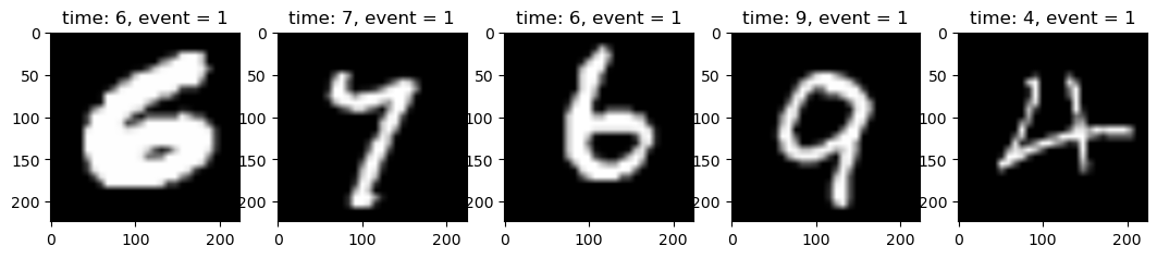
For this experiment, here’s are our assumptions: * We are using the MNIST dataset as inputs. * The observed digits becomes the time to event (e.g., the picture of a nine becomes time=9). * To prevent log(0) issue, all zeros are transformed as tens (time 0 -> 10) * All samples experienced an event (no censoring)

# Transforms our images
transforms = v2.Compose(
    [
        v2.ToImage(),
        v2.ToDtype(torch.float32, scale=True),
        v2.Resize(224, antialias=True),
        v2.Normalize(mean=(0,), std=(1,)),
    ]
)

torch.manual_seed(42)

# Load datamodule
datamodule = MNISTDataModule(batch_size=BATCH_SIZE, transforms=transforms)
datamodule.prepare_data()  # Download the data
datamodule.setup()  # Wrangle the data

# print image examples, with label
x, y = next(iter(datamodule.train_dataloader()))

plt.rcParams["figure.figsize"] = [13, 5]
for i in range(5):
    plt.subplot(1, 5, i + 1)
    plt.imshow(x[i].squeeze(), cmap="gray")
    plt.title(f"time: {y[i]}, event = 1")

Setup model backbone

First we need to define out model backbone. We will use the resnet18 model, without pretrained weights. We change two aspect of the model to fit our experiment:

• Changed the first convolution layer to fit our grayscale images

• Changed the last dense layer to output a single value (here log hazard)

resnet = resnet18(weights=None)
# Fits grayscale images
resnet.conv1 = torch.nn.Conv2d(
    1, 64, kernel_size=(7, 7), stride=(2, 2), padding=(3, 3), bias=False
)
# Output log hazards
resnet.fc = torch.nn.Linear(in_features=resnet.fc.in_features, out_features=1)

# Sanity checks
x = torch.randn((6, 1, 28, 28))  # Example batch of 6 MNIST images
print(f"{transforms(x).shape}")  # Check input dimension
print(f"{resnet(transforms(x)).shape}")  # Check output dimension

torch.Size([6, 1, 224, 224])
torch.Size([6, 1])

Regular model training

For this experiment, we are using the trainer from pytorch lightning. Most of the boilerplate code is under the hood, so we can focus on the ease of using the TorchSurv loss.

# Train first model (regular training) using our backbone
model_regular = LitMNIST(backbone=resnet)

# Define trainer
trainer = L.Trainer(
    accelerator="auto",  # Use best accelerator
    logger=False,  # No logging
    enable_checkpointing=False,  # No model checkpointing
    limit_train_batches=0.1,  # Train on 10% of data
    max_epochs=EPOCHS,  # Train for EPOCHS
    fast_dev_run=FAST_DEV_RUN,
    deterministic=True,
)

GPU available: True (mps), used: True
TPU available: False, using: 0 TPU cores
IPU available: False, using: 0 IPUs
HPU available: False, using: 0 HPUs

# Fit the model
trainer.fit(model_regular, datamodule)

  | Name  | Type   | Params
---------------------------------
0 | model | ResNet | 11.2 M
---------------------------------
11.2 M    Trainable params
0         Non-trainable params
11.2 M    Total params
44.683    Total estimated model params size (MB)

Epoch 1: 100%|██████████| 11/11 [01:02<00:00,  0.18it/s, loss_step=218.0, val_loss_step=282.0, cindex_step=0.652, val_loss_epoch=287.0, cindex_epoch=0.665, loss_epoch=228.0]

`Trainer.fit` stopped: `max_epochs=2` reached.

Epoch 1: 100%|██████████| 11/11 [01:02<00:00,  0.18it/s, loss_step=218.0, val_loss_step=282.0, cindex_step=0.652, val_loss_epoch=287.0, cindex_epoch=0.665, loss_epoch=228.0]

# Test the model
trainer.test(model_regular, datamodule)

Testing DataLoader 0: 100%|██████████| 20/20 [01:22<00:00,  0.24it/s]
────────────────────────────────────────────────────────────────────────────────────────────────────────────────────────
       Test metric             DataLoader 0
────────────────────────────────────────────────────────────────────────────────────────────────────────────────────────
      cindex_epoch          0.6686268448829651
     val_loss_epoch         -458.2862548828125
────────────────────────────────────────────────────────────────────────────────────────────────────────────────────────

[{'val_loss_epoch': -458.2862548828125, 'cindex_epoch': 0.6686268448829651}]

Momentum

For the the last part of the experiment, we are using the same backbone model, but now using a momentum loss. This loss allows to use previously computed batch value to increasing the effective loss samples. Details can be found here.

The idea behind is fairly simple and inspired from MoCo to fit into a survival analysis.

FACTOR = 10  # Number of batch to keep in memory. Increase our training batch size artificially by factor of 10 here
resnet_momentum = Momentum(resnet, neg_partial_log_likelihood, steps=FACTOR, rate=0.999)
model_momentum = LitMomentum(backbone=resnet_momentum)

# By using momentum, we can in theory reduce our batch size by factor and still have the same effective sample size
datamodule_momentum = MNISTDataModule(
    batch_size=BATCH_SIZE // FACTOR, transforms=transforms
)

# Define trainer
trainer = L.Trainer(
    accelerator="auto",  # Use best accelerator
    logger=False,  # No logging
    enable_checkpointing=False,  # No model checkpointing
    limit_train_batches=0.1,  # Train on 10% of data
    max_epochs=EPOCHS,  # Train for EPOCHS
    fast_dev_run=FAST_DEV_RUN,
    deterministic=True,
)
# Fit the model
trainer.fit(model_momentum, datamodule_momentum)

GPU available: True (mps), used: True
TPU available: False, using: 0 TPU cores
IPU available: False, using: 0 IPUs
HPU available: False, using: 0 HPUs

  | Name  | Type     | Params
-----------------------------------
0 | model | Momentum | 22.3 M
-----------------------------------
11.2 M    Trainable params
11.2 M    Non-trainable params
22.3 M    Total params
89.366    Total estimated model params size (MB)

Epoch 1: 100%|██████████| 110/110 [01:18<00:00,  1.40it/s, loss_step=57.10, val_loss_step=63.80, cindex_step=0.848, val_loss_epoch=59.80, cindex_epoch=0.841, loss_epoch=58.10]

`Trainer.fit` stopped: `max_epochs=2` reached.

Epoch 1: 100%|██████████| 110/110 [01:18<00:00,  1.40it/s, loss_step=57.10, val_loss_step=63.80, cindex_step=0.848, val_loss_epoch=59.80, cindex_epoch=0.841, loss_epoch=58.10]

# Validate the model
trainer.test(model_momentum, datamodule_momentum)

Testing DataLoader 0: 100%|██████████| 200/200 [01:38<00:00,  2.03it/s]
────────────────────────────────────────────────────────────────────────────────────────────────────────────────────────
       Test metric             DataLoader 0
────────────────────────────────────────────────────────────────────────────────────────────────────────────────────────
      cindex_epoch           0.858147144317627
     val_loss_epoch          72.23859405517578
────────────────────────────────────────────────────────────────────────────────────────────────────────────────────────

[{'val_loss_epoch': 72.23859405517578, 'cindex_epoch': 0.858147144317627}]

# Setup metics for each model
from torchsurv.metrics.cindex import ConcordanceIndex

cindex1 = ConcordanceIndex()  # Regular model
cindex2 = ConcordanceIndex()  # Momentum model

# Infere log hazards on unseen batch from test data
model_regular.eval()
model_momentum.eval()
with torch.no_grad():
    x, y = next(iter(datamodule.test_dataloader()))
    y[y == 0] = 10
    log_hz1 = model_regular(x)
    # For momentum, we advice to use the target network for inteference
    log_hz2 = model_momentum.model.target(x)

Despite training with batches 10x smaller than the regular model, the momentum model is performing better than the regular model on the same test batch.

print(f"Cindex (regular)  = {cindex1(log_hz1, torch.ones_like(y).bool(), y.float())}")
print(f"Cindex (momentum) = {cindex2(log_hz2, torch.ones_like(y).bool(), y.float())}")
# H1: cindex_momentum > cindex_regular, H0: same
print(f"Compare (p-value) = {cindex2.compare(cindex1)}")

Cindex (regular)  = 0.6948477029800415
Cindex (momentum) = 0.8578558564186096
Compare (p-value) = 2.1650459203215178e-11