Robustify Mixture Priors

Add a non-informative component to a mixture prior.

Usage

robustify(priormix, weight, mean, n = 1, ...)

# S3 method for class 'betaMix'
robustify(priormix, weight, mean, n = 1, ...)

# S3 method for class 'gammaMix'
robustify(priormix, weight, mean, n = 1, ...)

# S3 method for class 'normMix'
robustify(priormix, weight, mean, n = 1, ..., sigma)

Arguments

priormix: orior (mixture of conjugate distributions).
weight: weight given to the non-informative component (0 < weight < 1).
mean: mean of the non-informative component. It is recommended to set this parameter explicitly.
n: number of observations the non-informative prior corresponds to, defaults to 1.
...: optional arguments are ignored.
sigma: Sampling standard deviation for the case of Normal mixtures.

Value

New mixture with an extra non-informative component named robust.

Details

It is recommended to robustify informative priors derived with gMAP using unit-information priors . This protects against prior-data conflict, see for example Schmidli et al., 2015.

The procedure can be used with beta, gamma and normal mixture priors. A unit-information prior (see Kass and Wasserman, 1995) corresponds to a prior which represents the observation of n=1 at the null hypothesis. As the null is problem dependent we strongly recommend to make use of the mean argument accordingly. See below for the definition of the default mean.

The weights of the mixture priors are rescaled to (1-weight) while the non-informative prior is assigned the weight given.

Methods (by class)

robustify(betaMix): The default mean is set to 1/2 which represents no difference between the occurrence rates for one of the two outcomes. As the uniform Beta(1,1) is more appropriate in practical applications, RBesT uses n+1 as the sample size such that the default robust prior is the uniform instead of the Beta(1/2,1/2) which strictly defined would be the unit information prior in this case.
robustify(gammaMix): The default mean is set to the mean of the prior mixture. It is strongly recommended to explicitly set the mean to the location of the null hypothesis.
robustify(normMix): The default mean is set to the mean of the prior mixture. It is strongly recommended to explicitly set the mean to the location of the null hypothesis, which is very often equal to 0. It is also recommended to explicitly set the sampling standard deviation using the sigma argument.

References

Schmidli H, Gsteiger S, Roychoudhury S, O'Hagan A, Spiegelhalter D, Neuenschwander B. Robust meta-analytic-predictive priors in clinical trials with historical control information. Biometrics 2014;70(4):1023-1032.

Kass RE, Wasserman L A Reference Bayesian Test for Nested Hypotheses and its Relationship to the Schwarz Criterion J Amer Statist Assoc 1995; 90(431):928-934.

Examples

bmix <- mixbeta(inf1=c(0.2, 8, 3), inf2=c(0.8, 10, 2))
plot(bmix)

rbmix <- robustify(bmix, weight=0.1, mean=0.5)
rbmix
#> Univariate beta mixture
#> Mixture Components:
#>   inf1  inf2  robust
#> w  0.18  0.72  0.10 
#> a  8.00 10.00  1.00 
#> b  3.00  2.00  1.00 
plot(rbmix)


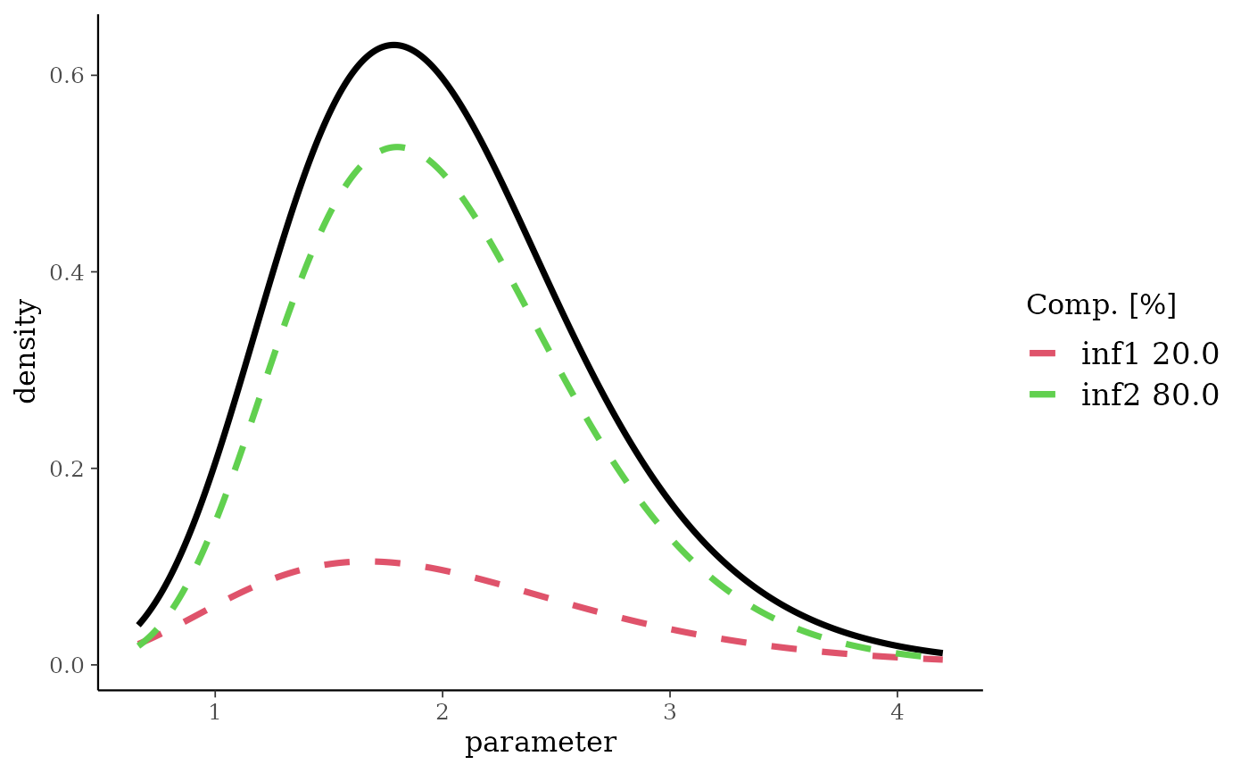
gmnMix <- mixgamma(inf1=c(0.2, 2, 3), inf2=c(0.8, 2, 5), param="mn")
plot(gmnMix)

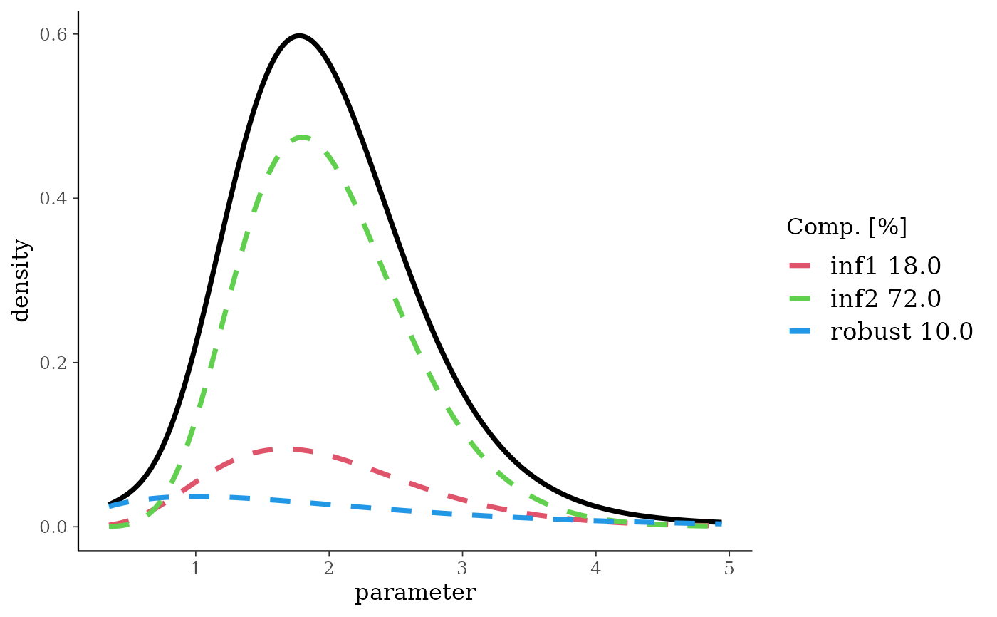
rgmnMix <- robustify(gmnMix, weight=0.1, mean=2)
rgmnMix
#> Univariate Gamma mixture
#> Mixture Components:
#>   inf1  inf2  robust
#> w  0.18  0.72  0.10 
#> a  6.00 10.00  2.00 
#> b  3.00  5.00  1.00 
plot(rgmnMix)


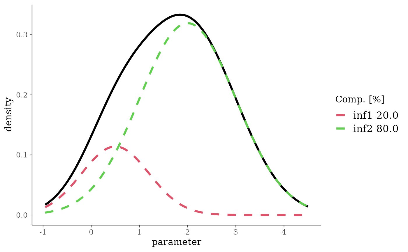
nm <- mixnorm(inf1=c(0.2, 0.5, 0.7), inf2=c(0.8, 2, 1), sigma=2)
plot(nm)

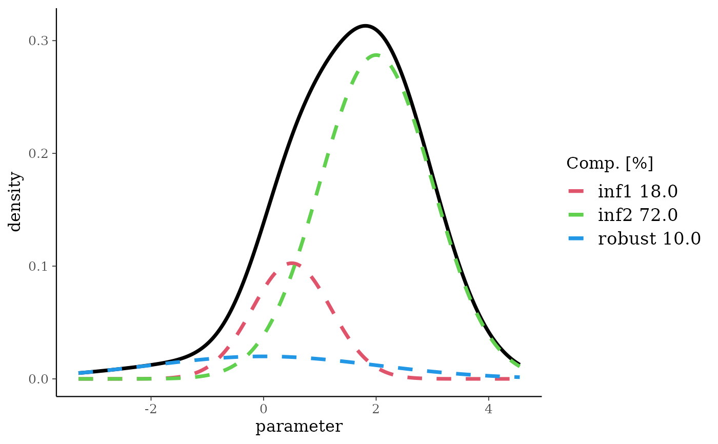
rnMix <- robustify(nm, weight=0.1, mean=0, sigma=2)
rnMix
#> Univariate normal mixture
#> Reference scale: 2
#> Mixture Components:
#>   inf1 inf2 robust
#> w 0.18 0.72 0.10  
#> m 0.50 2.00 0.00  
#> s 0.70 1.00 2.00  
plot(rnMix)