---
author:
- Sebastian Weber - <sebastian.weber@novartis.com>
bibliography: references.bib
---
<!-- https://raw.githubusercontent.com/Novartis/bamdd/main/src/_macros.qmd -->
{{< include _macros.qmd >}}
# Model setup & priors {#sec-model-priors}
```{r, eval=TRUE,echo=TRUE,message=FALSE,warning=FALSE,cache=FALSE}
#| code-fold: true
#| code-summary: "Show R setup"
library(ggplot2)
library(dplyr)
library(knitr)
library(brms)
library(posterior)
library(ggdist)
library(bayesplot)
library(tidybayes)
library(forcats)
library(RBesT)
here::i_am("src/01c_priors.qmd")
# instruct brms to use cmdstanr as backend and cache all Stan binaries
options(brms.backend="cmdstanr", cmdstanr_write_stan_file_dir=here::here("_brms-cache"))
# create cache directory if not yet available
dir.create(here::here("_brms-cache"), FALSE)
set.seed(593467)
theme_set(theme_bw(12))
```
```{r, include=FALSE, echo=FALSE, eval=TRUE, cache=FALSE}
# invisible to the reader additional setup steps, which are optional
source(here::here("src", "setup.R"))
```
Within the Bayesian regression modeling in Stan framework `brms`
priors are required to perform inference. This introductory material
is intended to provide some pragmatic considerations on how to setup
priors and point readers to material to follow-up on. The case studies
themselves provide details on setting up priors for the respective
problem. By default these priors have been chosen to have minimal
impact on the posterior whenever appropriate and also ensure stable
numerical inference. As a consequence, the results from the case
studies will resemble respective Frequentist model results in most
cases. Nonetheless, priors are defined explicitly for all models,
since these are an integral part of any Bayesian analysis. This can be
easily seen by considering Bayes rule to obtain the posterior:
$$ p(\theta | y) = \frac{p(y|\theta) \, p(\theta)}{p(y)} \propto p(y|\theta) \, p(\theta)$$
The marginal likelihood term $p(y)$ can be dropped, since this is
merely a normalization constant given that we condition the inference
on the observed data $y$. What is left is hence the product of the
likelihood $p(y|\theta)$ multiplied by the prior $p(\theta)$. The
posterior information on $\theta$ is hence provided equally by
likelihood and prior.
From a practical perspective one may ask under which circumstances it
actually matters which prior we set. In many cases the posterior is
dominated by the data, which means that the likelihood term
$p(y|\theta)$ is much larger than the prior term $p(\theta)$. This is
the case for most case studies. It is tempting to drop the prior in
these cases and not worry about it. However, this is not recommended
as it is in many instances of interest to study a model with small
sample sizes eventually (by applying the model to subsets, increasing
model complexity, etc.). Another practical aspect is the numerical
stability and quality of the Markov Chain Monte Carlo (MCMC) sample we
obtain from Stan. Without a prior the inference problem becomes much
harder to solve. That is, the Markov Chain Monte Carlo (MCMC) sampler
Stan has to consider the full sampling space of the prior. Dropping
the prior entirely implies an improper prior on the sampling space
which becomes un-countably infinitely large. Rather than dropping the
prior entirely we strongly recommend to consider so-called weakly
informative priors. While no formal definition is given in the
literature, these priors aim to identify the *scale* of
parameters. This requires a basic understanding of the parameters for
which priors are being defined. Thus, a prior can only be understood
in the overall context of the likelihood, parametrization and problem
at hand [see also @Gelman2017]. For most statistical analyses this
means to consider the endpoint and the applied transformations.
<!--
A notable exception to this are the case studies on the meta
analytic predictive (MAP) priors. These case studies infer between
study heterogeneity from very few studies and therefore the prior used
for the heterogeneity parameter will not be dominated by the data. The
MAP priors themselves represent *data* derived priors and they have
become very popular nowadays.
-->
To just get started with `brms` one may choose to not specify priors
when calling `brm`. Doing so will let `brms` provide in most cases
reasonable default priors. These default priors are intended to avoid
any influence on the calculated posterior. Hence, the results are
fully data driven and will be very close to the respective Frequentist
maximum likelihood inference result. However, the default prior is not
guaranteed to stay stable between releases and can thus change whenever
the `brms` version changes.
Given that any Bayesian analysis requires a prior, we recommend to
always explicitly define these - even if these just repeat the default
prior from `brms`, which one can easily obtain. Here we use as example
binomially distributed data (responder in a control arm) and we use
the simplest possible model, which will pool the information across the
different studies (in practice one would allow for between-trial
heterogeneity):
```{r}
model <- bf(r | trials(n) ~ 1, family=binomial)

## with brms >= 2.21.0 we can  directly write...
## default_prior(model, data=RBesT::AS)

## a workaround is to create an empty brms model and obtain the
## defined prior like
prior_summary(brm(model, data=RBesT::AS, empty=TRUE)) |> kable()
```
Note that we have defined first the model via the `bf` call. This
defines the linear predictor and the likelihood using the `family`
argument of `bf`. We recommend to always explicitly do this step first
as it defines the likelihood and the model parametrization in one
step. Choosing these is a critical first step in defining the model
and, most importantly, the chosen priors can only be understood in the
context of the model (likelihood and parametrization) [see @Gelman2017].
Rather than running the model with no explicit prior definition we
encourage users to explicitly define the priors used for the
analysis - even if these are simply the default priors:
```{r warning=FALSE, message=FALSE}
model_def <- bf(r | trials(n) ~ 1, family=binomial)
model_prior <- prior(student_t(3, 0, 2.5), class=Intercept)

fit <- brm(model_def, data=RBesT::AS, prior=model_prior, seed=467657, refresh=0)
fixef(fit)
```
The provided default prior is indeed not informative, as can be seen
by comparing the posterior estimate to the respective Frequentist fit
from `glm`:
```{r warning=FALSE, message=FALSE}
fit_freq <- glm(cbind(r, n-r) ~ 1, data=RBesT::AS, family=binomial)
## intercept estimate
coef(fit_freq)
## standard error estimate
sqrt(vcov(fit_freq)[1,1])
```
In this case the data with a total of `r sum(RBesT::AS$n)` subjects
dominates the posterior. Nonetheless, it is illustrative to consider in
more detail the prior here as an example. Importantly, the intercept
of the model is defined on the *logit* scale of the response
probability as it is common for a standard logistic regression. The
transformation changes the scale from the interval 0 to 1 to a new
scale which covers the entire space of reals. While formally very
large or very small logits are admissible, the range from 5% to 95%
response rate corresponds to -3 to 3 on the logit space
approximately. Thus, logit values smaller or greater than these values
would be considered extreme effects.
When defining a prior for a model we would typically want to compare
different choices of the prior to one another. As example prior for
the intercept only model we may compare here three different priors:
(i) a very wide prior $\N(0,10^2)$, (2) the default `brms` prior and
(3) the density $\N(0,2^2)$ as used as default prior in `RBesT` for
this problem. In a first step we sample these priors and assess them
graphically. We could use `brms` to sample these priors directly with
the argument `sample_prior="only"`, but we instead use basic R
functions for simplicity:
```{r warning=FALSE, message=FALSE}
#| code-fold: true
#| code-summary: "Show the code"
num_draws <- 1E4
priors_cmp <- tibble(case=c("wide", "brms", "RBesT"),
                     density=c("N(0,10^2)", "S(3, 0, 2.5^2)", "N(0, 2^2)"),
                     prior=rvar(cbind(rnorm(num_draws, 0, 10),
                                      rstudent_t(num_draws, 3, 0, 2.5),
                                      rnorm(num_draws, 0, 2))))

kable(priors_cmp, digits=2)
priors_logit <- priors_cmp |>
    ggplot(aes(y=case, xdist=prior)) +
    stat_slab() +
    xlab("Intercept\nlinear predictor") +
    ylab(NULL) +
    labs(title="Prior logit scale") +
    coord_cartesian(xlim=c(-30, 30))

priors_response <- priors_cmp |>
    ggplot(aes(y=case, xdist=rdo(inv_logit(prior)))) +
    stat_slab() +
    xlab("Intercept\nresponse scale") +
    ylab(NULL) +
    labs(title="Prior response scale") +
    coord_cartesian(xlim=c(0, 1))

bayesplot_grid(priors_logit, priors_response, grid_args=list(nrow=1))
```
As one can easily see, the wide prior has density at very extreme
logit values of -20 and 20. In comparison, the `brms` and the `RBesT`
default prior place most probability mass in the vicinity of
zero. While the wide prior may suggest to be very non-informative it's
meaning becomes clearer when back transforming to the original
response scale from 0 to 1. It is clear that the wide prior implies
that we expect extreme response rates of either 0 or 1. In contrast,
the `RBesT` default prior has an almost uniform distribution on the 0
to 1 range while the default `brms` prior has some "U" shape. To now
further discriminate these priors a helpful concept is to consider
**interval probabilities** for pre-defined categories. The definition
of cut-points of the categories is problem specific, but can be
defined with usual common sense for most endpoints. The critical step
here is in defining these categories and documenting these along with
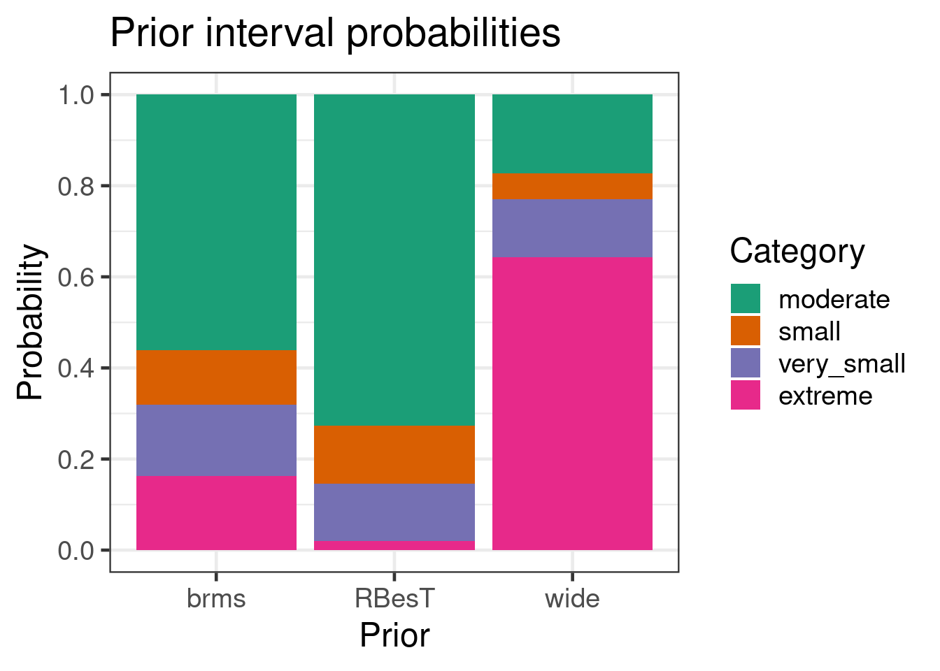
the analysis. Here we categorize the response as extreme 0-1% &
99-100%, very small 1-5% & 95-99%, small 5-10% & 90-95% and
moderate for the remainder. Comparing then these priors gives:
```{r warning=FALSE, message=FALSE}
#| code-fold: true
#| code-summary: "Show the code"
response_category <- function(r) {
    fct_rev(cut(pmin(r, 1-r), c(0, 0.01, 0.05, 0.1, 0.5), labels=c("extreme", "very_small", "small", "moderate")))
}

priors_cmp |> unnest_rvars()|>
    ggplot(aes(x=case, fill=response_category(inv_logit(prior)))) +
    geom_bar(position="fill") +
    xlab("Prior") +
    ylab("Probability") +
    labs(title="Prior interval probabilities", fill="Category") +
    scale_y_continuous(breaks=seq(0,1,by=0.2)) +
    theme(legend.position="right")
mutate(priors_cmp,
       prior_response=rfun(inv_logit)(prior),
       summarise_draws(prior_response,
                       extreme=~100*E(.x < 0.01 | .x > 0.99),
                       very_small=~100*E( (0.01 <= .x & .x < 0.05) | (0.95 < .x & .x <= 0.99) ),
                       small=~100*E( (0.05 <= .x & .x < 0.1) | (0.9 < .x & .x <= 0.95) ),
                       moderate=~100*E( (0.1 <= .x & .x < 0.9) )
                       )) |>
    select(case, density, extreme, very_small, small, moderate) |>
    kable(digits=1, caption="Interval probabilities per prior given in percent")
```
It is apparent that the seemingly non-informative prior "wide" is in
fact an informative prior implying that the expected response rates
are extreme. This is the consequence of transforming to the logit
scale.
In practice one would most certainly not fit the intercept only model,
which pools the information. The `RBesT::AS` data set is in fact the
standard example for the use of historical control data.
```{r warning=FALSE, message=FALSE}
kable(RBesT::AS)
```
To use this data as historical control data one uses instead of the
intercept only model a random intercept model, which casts this
into a meta-analtyic model:
```{r warning=FALSE, message=FALSE}
model_meta_def <- bf(r | trials(n) ~ 1 + (1 | study), family=binomial)
model_meta_prior <- prior(normal(0, 2), class=Intercept) +
    prior(normal(0, 0.5), class=sd, coef=Intercept, group=study)

fit_meta <- brm(model_meta_def, data=RBesT::AS, prior=model_meta_prior,
                seed=982345, refresh=0, control=list(adapt_delta=0.95))
summary(fit_meta)
```
The meta-analytic model is generative in the sense of allowing to
predict the mean response rate for future studies by way of the
hierarchical model structure. Now the importance of the prior on the
overall intercept becomes more relevance as the information from each
study is discounted through the random effects model leading to less
data to estimate the parameter in comparison to the full pooling
model. However, the key parameter in this model is the between-trial
heterogeneity parameter. In the example a half-normal prior with scale
1 is used (`brms` knows that the parameter must be positive and hence
truncates the prior at zero automatically). This distribution of a
half-normal density has been studied extensively in the literature and
found to be a robust choice in a wide range of problems. For this
reason, it is a very rational choice to use this prior in the current
(and future) analyses. The choice of the scale of 0.5 is often
referred to as a conservative choice in this problem while 1 is a very
conservative choice and 0.25 a less conservative choice. A
complication with the hierarchical model is that $\tau$ itself implies
a distribution. To simplify this, we first consider the case of a
known between-trial heterogeneity parameter and study what this
implies. For a known $\tau$ the range of implied log odds can be
characterized by the respective 95% probability mass range given by $2
\cdot 1.96 \, \tau$, which is interpret-able as the largest log odds
ratio. Recalling that the between-study heterogeneity parameter
controls the (random) differences in the logits of response rates
between studies, it is helpful to consider the distribution of implied
log odds ratios between random pairs of two studies. These differences
(log odds ratios) have a distribution of $\N(0, (\sqrt{2} \,
\tau)^2)$. Considering the absolute value of these differences, the
distributions becomes a half-normal with scale $\sqrt{2} \, \tau$,
which has it's median value at $1.09 \, \tau$. This results for a
range of values of $\tau$ on the respective odds scale to:
```{r echo=FALSE}
tau_known <- tibble(tau=c(0, 0.125, 0.25, 0.5, 1.0, 1.5, 2)) |>
mutate(largest_odds_ratio=exp(3.92 * tau),
median_odds_ratio=exp(1.09 * tau))
tau_known |> kable(digits=3)
```
In [@Neuenschwander2020] suggest the categorization of the
between-study heterogeneity $\tau$ parameter the values of $1$ for
being large, $0.5$ substantial, $0.25$ moderate, and $0.125$
small. Considering these with the table above qualifies these
categories as plausible. An alternative approach to the categorization
is to consider what is an extreme value for $\tau$ (like unity) and
then choose the prior on $\tau$ such that a large quantile (like the
95% quantile) corresponds to this extreme value.
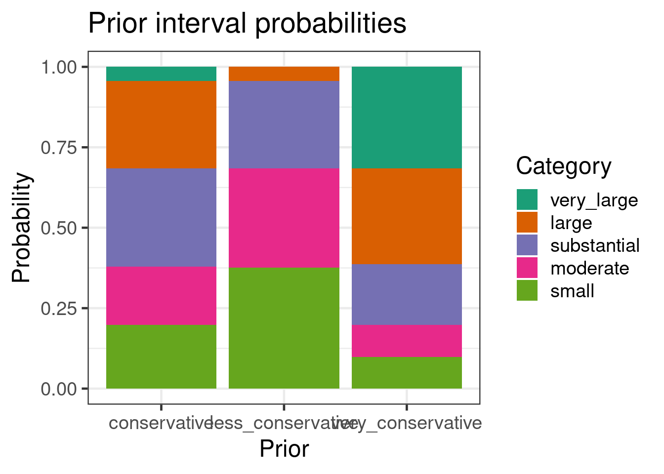
With the categorization of specific values for $\tau$ we can now
proceed and consider the interval probabilities for these categories
for the different choices of $\tau \sim \HN(s^2)$ for $s=1$ and
$s=1/2$.
```{r}
#| code-fold: true
#| code-summary: "Show the code"
priors_cmp_tau <- tibble(case=c("less_conservative", "conservative", "very_conservative"),
                         density=c("HN(0, (1/4)^2)", "HN(0, (1/2)^2)", "HN(0, 1^2)"),
                         prior=rvar(cbind(abs(rnorm(num_draws, 0, 0.25)),
                                          abs(rnorm(num_draws, 0, 0.5)),
                                          abs(rnorm(num_draws, 0, 1))))
                         )

kable(priors_cmp_tau)
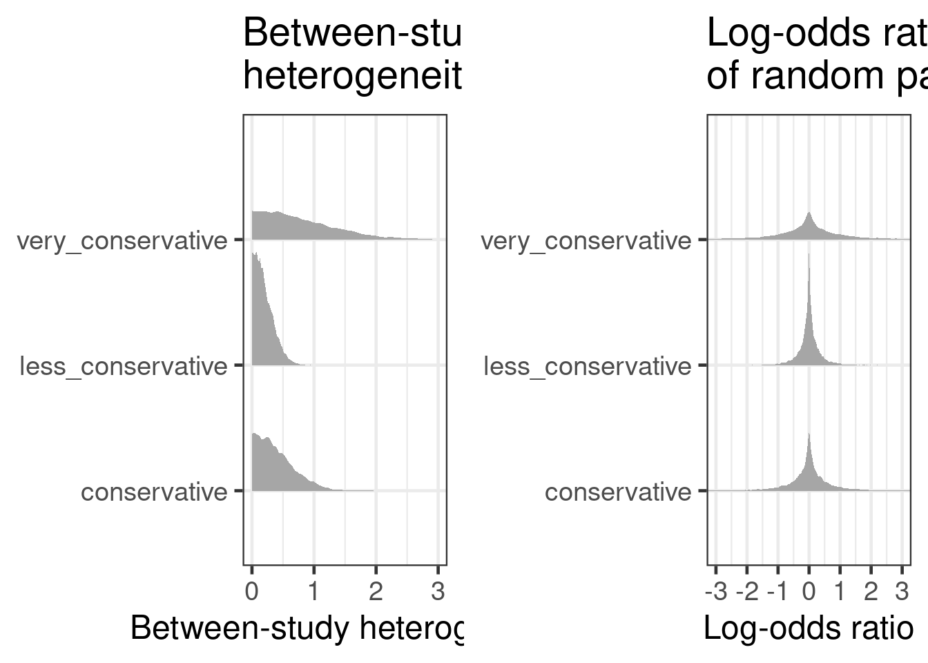
priors_hetero <- priors_cmp_tau |>
    ggplot(aes(y=case, xdist=prior)) +
    stat_slab() +
    xlab("Between-study heterogeneity") +
    ylab(NULL) +
    scale_x_continuous(breaks=0:3) +
    labs(title="Between-study\nheterogeneity") +
    coord_cartesian(xlim=c(0, 3))

priors_lor <- priors_cmp_tau |>
    mutate(lor1=rvar_rng(rnorm, n=n(), mean=0, prior),
           lor2=rvar_rng(rnorm, n=n(), mean=0, prior)) |>
    ggplot(aes(y=case, xdist=lor1-lor2)) +
    stat_slab() +
    xlab("Log-odds ratio") +
    ylab(NULL) +
    scale_x_continuous(breaks=-5:5) +
    labs(title="Log-odds ratio\nof random pair") +
    coord_cartesian(xlim=c(-3, 3))

bayesplot_grid(priors_hetero, priors_lor, grid_args=list(nrow=1))
```
```{r warning=FALSE, message=FALSE}
#| code-fold: true
#| code-summary: "Show the code"
tau_category <- function(tau) {
    fct_rev(cut(tau, c(0, 0.125, 0.25, 0.5, 1, Inf), labels=c("small", "moderate", "substantial", "large", "very_large")))
}

priors_cmp_tau |> unnest_rvars()|>
    ggplot(aes(x=case, fill=tau_category(prior))) +
    geom_bar(position="fill") +
    xlab("Prior") +
    ylab("Probability") +
    labs(title="Prior interval probabilities", fill="Category") +
    ##scale_y_continuous(breaks=seq(0,1,by=0.2)) +
    theme(legend.position="right")
mutate(priors_cmp_tau,
       summarise_draws(prior,
                       small=~100*E(.x < 0.125),
                       moderate=~100*E( 0.125 <= .x & .x < 0.25 ),
                       substantial=~100*E( 0.25 <= .x & .x < 0.5 ),
                       large=~100*E( 0.5 <= .x & .x < 1 ),
                       very_large=~100*E( .x >= 1 )
                       )) |>
    select(case, density, small, moderate, substantial, large, very_large) |>
    kable(digits=1, caption="Interval probabilities per prior given in percent")
```
We can see that the "conservative" choice has an about 5% tail
probability exceeding the value of large. This implies that some
degree of homogeneity between the studies is given. This is usually
the case whenever meta-analyses are conducted, since the inclusion &
exclusion criteria for studies are aligned to a certain degree in
order to ensure that a similar patient population is included in the
analysis. In contrast, the "very conservative" choice admits with 30%
probability mass the possibility of values in the domain "very large"
for which practically no borrowing of historical information
occurs. The "less conservative" choice on the hand has 5% tail
probability above substantial. This way a large heterogeneity is
considered to be unlikely as it can be the case for twin Phase III
studies, for example.
Additional literature for consideration:
- Empirical priors study for HTA treatment effect evaluation by the
German IQWIG [@Lilienthal2023]
- Empirical priors for meta-analyses organized in disease specific
manner [@Turner2015]
- Endpoint specific considerations for between-trial heterogeneity
parameter priors in random effect meta-analyses [@Rover2021]
- Comprehensive introductory book to applied Bayesian data analysis
with detailed discussion on many examples [@Gelman2014]
- Live wiki document maintained by Stan user community (heavily
influenced by Andrew Gelman & Aki Vehtari) [@stanwikiPrior]
- Prior strategy based on nested modeling considerations (penalization
of more complex models), [@Simpson2014]
- Global model shrinkage regularized horseshoe prior [@Piironen2017]
or R2D2 prior (overall $R^2$) [@Zhang2022]
::: {.content-visible when-profile="dummy"}
## Further considerations
{{< video videos/brms3-hq-alt-2-priors.mp4 >}}
:::