Posterior of predictive

Simulation of the predictive distribution.

Usage

# S3 method for class 'blrmfit'
posterior_predict(object, newdata, draws, ...)

Arguments

object

fitted model object

newdata

optional data frame specifying for what to predict; if missing, then the data of the input model object is used

draws

number of returned posterior draws; by default the entire posterior is returned

...

not used in this function

Value

Matrix of dimensions draws by nrow(newdata) where row correspond to a draw of the posterior and each column corresponds to a row in newdata. The columns are labelled with the row.names of newdata.

Details

Simulates the posterior predictive of the model object for the specified data set.

Group and strata definitions

The groups and strata as defined when running the blrm_exnex analysis cannot be changed at a later stage. As a result no evaluations can be performed for groups which have not been present in the data set used for running the analysis. However, it is admissible to code the group (and/or stratum) column as a factor which contains empty levels. These groups are thus not contained in the fitting data set and they are assigned by default to the first stratum. In addition priors must be setup for these groups (and/or strata). These empty group (and/or strata) levels are then allowed in subsequent evaluations. This enables the evaluation of the hierarchical model in terms of representing a prior for future groups.

Examples

## Setting up dummy sampling for fast execution of example
## Please use 4 chains and 100x more warmup & iter in practice
.user_mc_options <- options(
  OncoBayes2.MC.warmup = 10, OncoBayes2.MC.iter = 20, OncoBayes2.MC.chains = 1,
  OncoBayes2.MC.save_warmup = FALSE
)


example_model("single_agent", silent = TRUE)
#> Warning: The largest R-hat is NA, indicating chains have not mixed.
#> Running the chains for more iterations may help. See
#> https://mc-stan.org/misc/warnings.html#r-hat
#> Warning: Bulk Effective Samples Size (ESS) is too low, indicating posterior means and medians may be unreliable.
#> Running the chains for more iterations may help. See
#> https://mc-stan.org/misc/warnings.html#bulk-ess
#> Warning: Tail Effective Samples Size (ESS) is too low, indicating posterior variances and tail quantiles may be unreliable.
#> Running the chains for more iterations may help. See
#> https://mc-stan.org/misc/warnings.html#tail-ess

post_pred <- posterior_predict(blrmfit)
## turn DLT counts into DLT rates
post_pred_rate <- sweep(post_pred, 2, hist_SA$num_patients, "/")

library(bayesplot)
library(ggplot2)

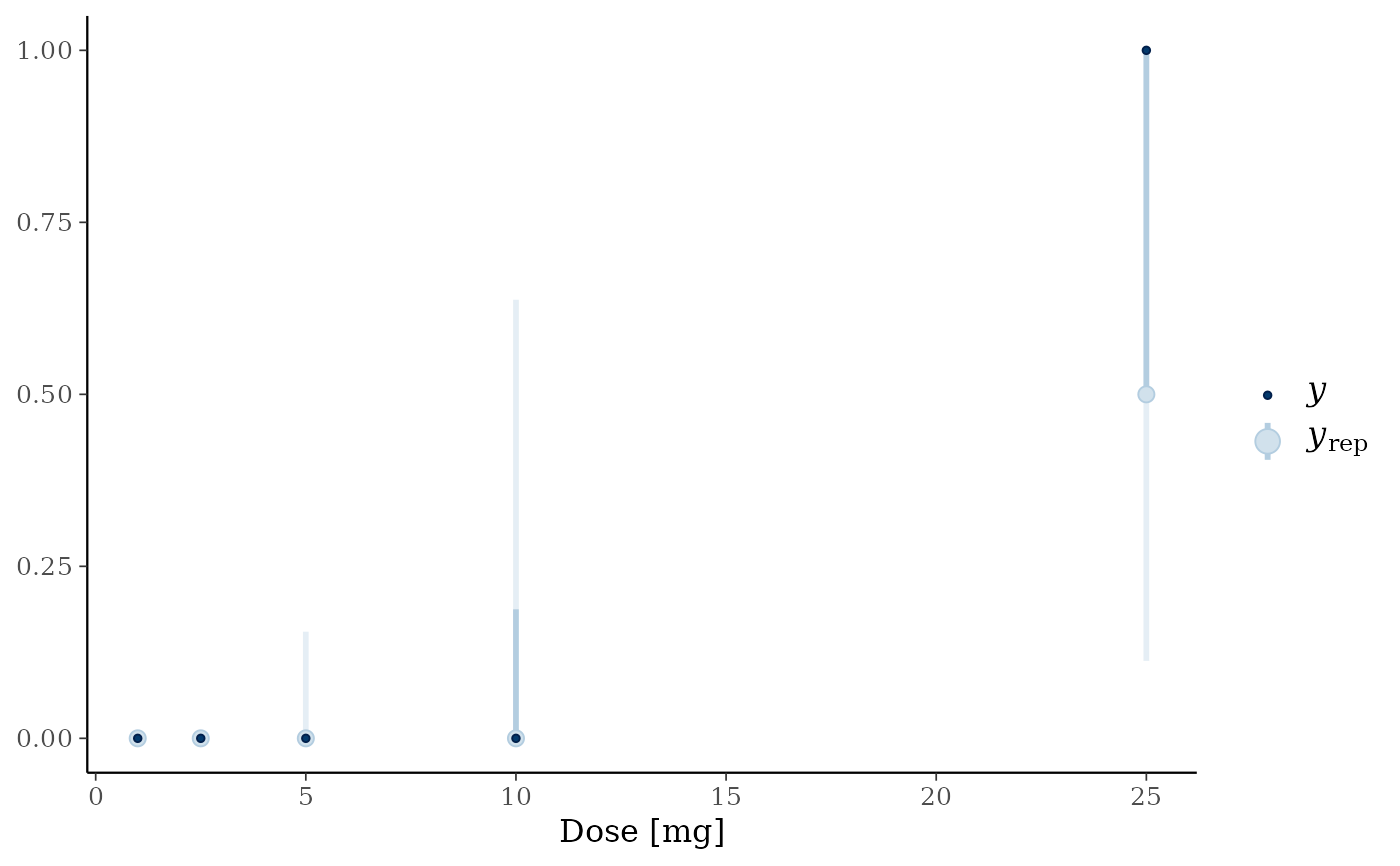
## compare posterior predictive of the model for the response rates
## with observed data
with(
  hist_SA,
  ppc_intervals(num_toxicities / num_patients, post_pred_rate, x = drug_A, prob_outer = 0.95)
) +
  xlab("Dose [mg]")


## Recover user set sampling defaults
options(.user_mc_options)