Posterior of linear predictor

Calculates the posterior of the linear predictor.

Usage

# S3 method for class 'blrmfit'
posterior_linpred(object, transform = FALSE, newdata, draws, ...)

Arguments

object

fitted model object

transform

logical (defaults to FALSE) indicating if the linear predictor on the logit link scale is transformed with inv_logit to the 0-1 response scale.

newdata

optional data frame specifying for what to predict; if missing, then the data of the input model object is used

draws

number of returned posterior draws; by default the entire posterior is returned

...

not used in this function

Value

Matrix of dimensions draws by nrow(newdata) where row correspond to a draw of the posterior and each column corresponds to a row in newdata. The columns are labelled with the row.names of newdata.

Details

Simulates the posterior of the linear predictor of the model object for the specified data set.

Group and strata definitions

The groups and strata as defined when running the blrm_exnex analysis cannot be changed at a later stage. As a result no evaluations can be performed for groups which have not been present in the data set used for running the analysis. However, it is admissible to code the group (and/or stratum) column as a factor which contains empty levels. These groups are thus not contained in the fitting data set and they are assigned by default to the first stratum. In addition priors must be setup for these groups (and/or strata). These empty group (and/or strata) levels are then allowed in subsequent evaluations. This enables the evaluation of the hierarchical model in terms of representing a prior for future groups.

Examples

## Setting up dummy sampling for fast execution of example
## Please use 4 chains and 100x more warmup & iter in practice
.user_mc_options <- options(
  OncoBayes2.MC.warmup = 10, OncoBayes2.MC.iter = 20, OncoBayes2.MC.chains = 1,
  OncoBayes2.MC.save_warmup = FALSE
)


## run single-agent analysis which defines blrmfit model object
example_model("single_agent", silent = TRUE)
#> Warning: The largest R-hat is NA, indicating chains have not mixed.
#> Running the chains for more iterations may help. See
#> https://mc-stan.org/misc/warnings.html#r-hat
#> Warning: Bulk Effective Samples Size (ESS) is too low, indicating posterior means and medians may be unreliable.
#> Running the chains for more iterations may help. See
#> https://mc-stan.org/misc/warnings.html#bulk-ess
#> Warning: Tail Effective Samples Size (ESS) is too low, indicating posterior variances and tail quantiles may be unreliable.
#> Running the chains for more iterations may help. See
#> https://mc-stan.org/misc/warnings.html#tail-ess

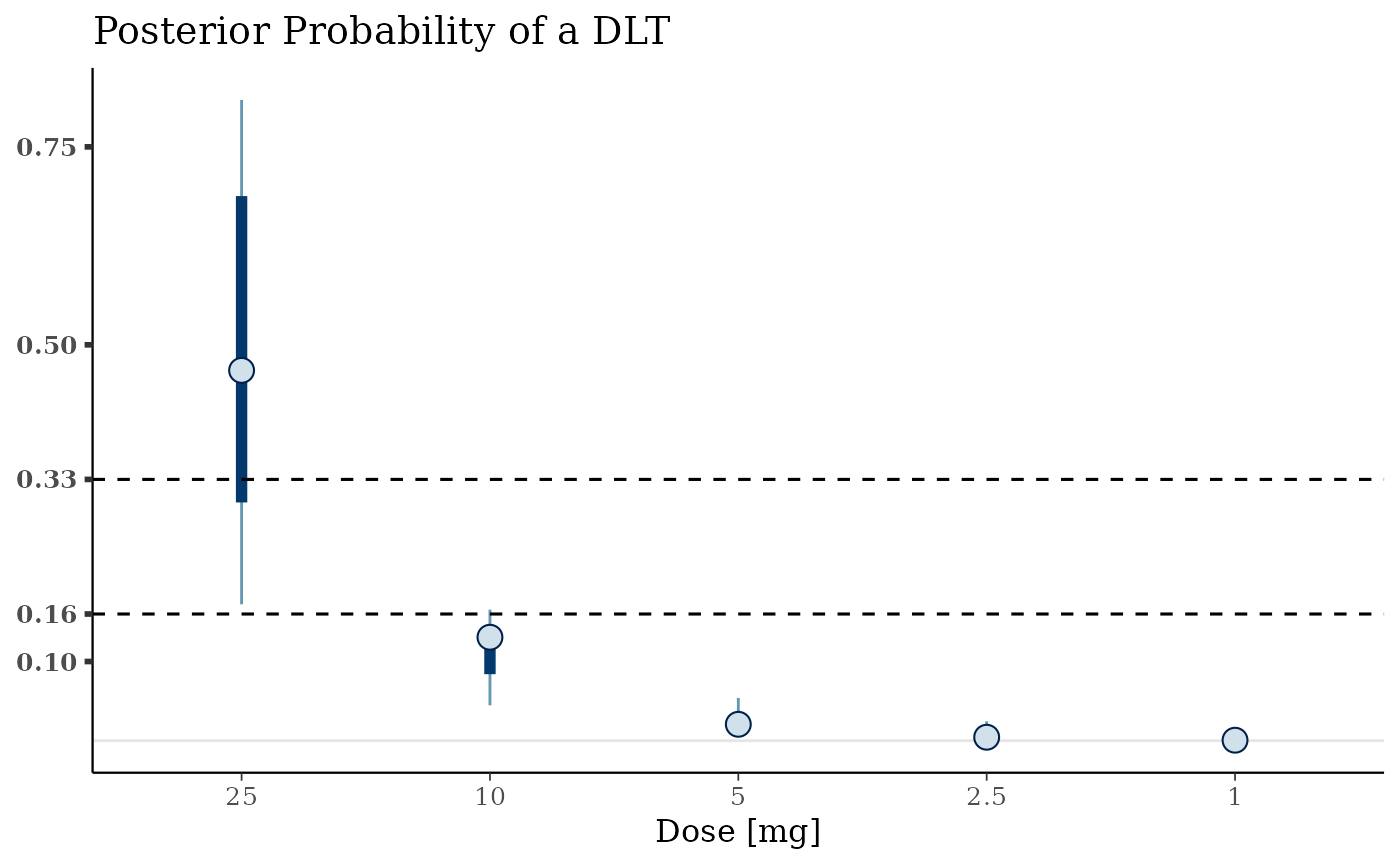
## obtain posterior of linear prediction on 0-1 scale
post_prob_dlt <- posterior_linpred(blrmfit, TRUE, newdata = hist_SA)
## name columns to obtain nice bayesplot labels
colnames(post_prob_dlt) <- hist_SA$drug_A

library(bayesplot)
#> This is bayesplot version 1.15.0
#> - Online documentation and vignettes at mc-stan.org/bayesplot
#> - bayesplot theme set to bayesplot::theme_default()
#>    * Does _not_ affect other ggplot2 plots
#>    * See ?bayesplot_theme_set for details on theme setting
library(ggplot2)
mcmc_intervals(post_prob_dlt, prob = 0.5, prob_outer = 0.95) +
  coord_flip() +
  vline_at(c(0.16, 0.33), linetype = 2) +
  ylab("Dose [mg]") +
  ggtitle("Posterior Probability of a DLT") +
  scale_x_continuous(breaks = c(0.1, 0.16, 0.33, 0.5, 0.75))
#> Scale for x is already present.
#> Adding another scale for x, which will replace the existing scale.


## Recover user set sampling defaults
options(.user_mc_options)