PD, Dose-Response - Ordinal
Alison Margolskee, Fariba Khanshan
Overview
This document contains exploratory plots for ordinal response data as well as the R code that generates these graphs. The plots presented here are based on simulated data (see: PKPD Datasets). Data specifications can be accessed on Datasets and Rmarkdown template to generate this page can be found on Rmarkdown-Template. You may also download the Multiple Ascending Dose PK/PD dataset for your reference (download dataset).
Ordinal data can be thought of as categorical data that has a natural order. For example, mild, moderate or severe. Another example could be Grade 1, Grade 2, Grade 3. Ordinal data can also come out of stratifying continuous data, for example binning a continuous variable into quartiles, or defining (arbitrary or meaningful) cutoffs for a continuous variable. Since ordinal data has a natural order, it is important to preserve that order when creating plots.
Setup
library(ggplot2)
library(dplyr)
library(tidyr)
library(gridExtra)
library(xgxr)

#flag for labeling figures as draft
status = "DRAFT"

## ggplot settings
xgx_theme_set()

#directories for saving individual graphs
dirs = list(
parent_dir = tempdir(),
rscript_dir  = "./",
rscript_name = "Example.R",
results_dir  = "./",
filename_prefix   = "",
filename     = "Example.png")
Load Dataset
pkpd_data <- read.csv("../Data/Multiple_Ascending_Dose_Dataset2.csv")

DOSE_CMT = 1
PD_CMT = 5
SS_PROFDAY = 6 # steady state prof day
PD_PROFDAYS = c(0, 2, 4, 6)

#ensure dataset has all the necessary columns
pkpd_data = pkpd_data %>%
  mutate(ID      = ID,     #ID   column
         TIME    = TIME,   #TIME column name
         NOMTIME = NOMTIME, #NOMINAL TIME column name
         PROFDAY = PROFDAY, #PROFILE DAY day associated with profile, e.g. day of dose administration
         LIDV    = LIDV,   #DEPENDENT VARIABLE column name
         CENS    = CENS,   #CENSORING column name
         CMT     = CMT,    #COMPARTMENT column
         DOSE    = DOSE,   #DOSE column here (numeric value)
         TRTACT  = TRTACT, #DOSE REGIMEN column here (character, with units),
         LIDV_UNIT = EVENTU,
         DAY_label = ifelse(PROFDAY > 0, paste("Day", PROFDAY), "Baseline"),
         ORDINAL_LEVELS = factor(case_when(
           CMT != PD_CMT ~ as.character(NA),
           LIDV == 1 ~ "Mild",
           LIDV == 2 ~ "Moderate",
           LIDV == 3 ~ "Severe"
         ), levels = c("Mild", "Moderate", "Severe"))
         )

#create a factor for the treatment variable for plotting
pkpd_data = pkpd_data %>%
  arrange(DOSE) %>%
  mutate(TRTACT_low2high      = factor(TRTACT, levels = unique(TRTACT)),
         TRTACT_high2low      = factor(TRTACT, levels = rev(unique(TRTACT))),
         ORDINAL_LEVELS_low2high    = ORDINAL_LEVELS,
         ORDINAL_LEVELS_high2low    = factor(ORDINAL_LEVELS, levels = rev(levels(ORDINAL_LEVELS))))

#create pd dataset
pd_data <- pkpd_data %>%
  filter(CMT == PD_CMT) %>%
  mutate(LIDV_jitter = jitter(LIDV, amount = 0.1),
         TIME_jitter     = jitter(TIME, amount = 0.1*24)
         )

#units and labels
time_units_dataset = "hours"
time_units_plot    = "days"
trtact_label       = "Dose"
time_label         = "Time (Days)"
dose_units         = unique((pkpd_data %>% filter(CMT == DOSE_CMT))$LIDV_UNIT) %>% as.character()
dose_label         = paste0("Dose (", dose_units, ")")
pd_units           = unique(pd_data$LIDV_UNIT) %>% as.character()
pd_ordinal_label   = paste0("Ordinal PD Marker (", pd_units, ")")
pd_response_label  = "Responder Rate (%)"
Provide an overview of the data
Percent of subjects by response category over time, faceted by dose
gg <- ggplot(data = pd_data, aes(x = factor(PROFDAY), fill = ORDINAL_LEVELS_high2low))
gg <- gg + geom_bar(position = "fill") + scale_y_continuous(labels = scales::percent)
gg <- gg + labs(x = time_label, y = pd_response_label)
gg <- gg + scale_fill_brewer(palette = 6)
gg <- gg + facet_grid(.~TRTACT_low2high)
gg <- gg + guides(fill = guide_legend(""))
gg <- gg + xgx_annotate_status(status)
gg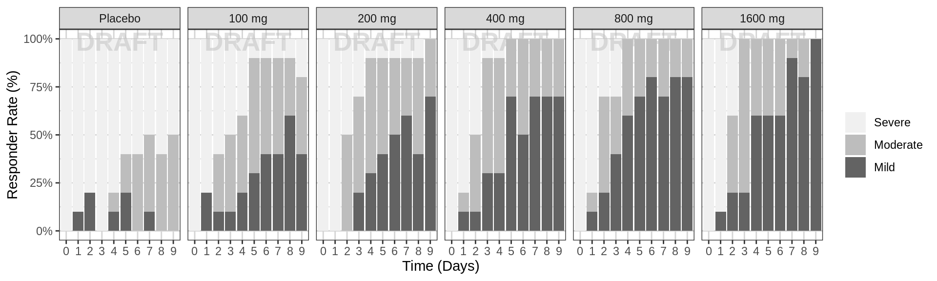
gg2 <- ggplot(data = pd_data, aes(x = PROFDAY, response = ORDINAL_LEVELS_high2low, color = ORDINAL_LEVELS_high2low))
gg2 <- gg2 + xgx_stat_ci(distribution = "ordinal",
                         geom = list("line", "point","errorbar"),
                         position = position_dodge(width = 12), alpha = 0.5)
gg2 <- gg2 + scale_y_continuous(labels = scales::percent)
gg2 <- gg2 + labs(x = time_label, y = pd_response_label)
gg2 <- gg2 + facet_grid(.~TRTACT_low2high)
gg2 <- gg2 + scale_fill_brewer(palette = 6)
gg2 <- gg2 + guides(color = guide_legend(""),fill = guide_legend(""))
gg2 <- gg2 + xgx_annotate_status(status)
gg2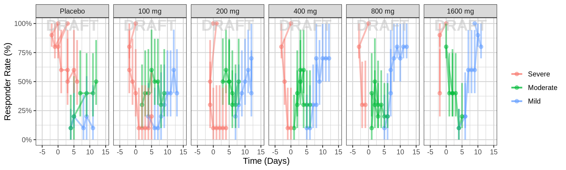
Percent of subjects by response category over time, colored by dose, faceted by response category
gg <- ggplot(data = pd_data, aes(x = PROFDAY, response = ORDINAL_LEVELS_high2low, color = TRTACT_low2high))
gg <- gg + xgx_stat_ci(distribution = "ordinal",
                         geom = list("line", "point","errorbar"),
                         position = position_dodge(width = 12), alpha = 0.5)
gg <- gg + scale_y_continuous(labels = scales::percent)
gg <- gg + labs(x = time_label, y = pd_response_label)
gg <- gg + facet_grid(ORDINAL_LEVELS_high2low~.)
gg <- gg + scale_fill_brewer(palette = 6)
gg <- gg + guides(color = guide_legend(""),fill = guide_legend(""))
gg <- gg + xgx_annotate_status(status)
gg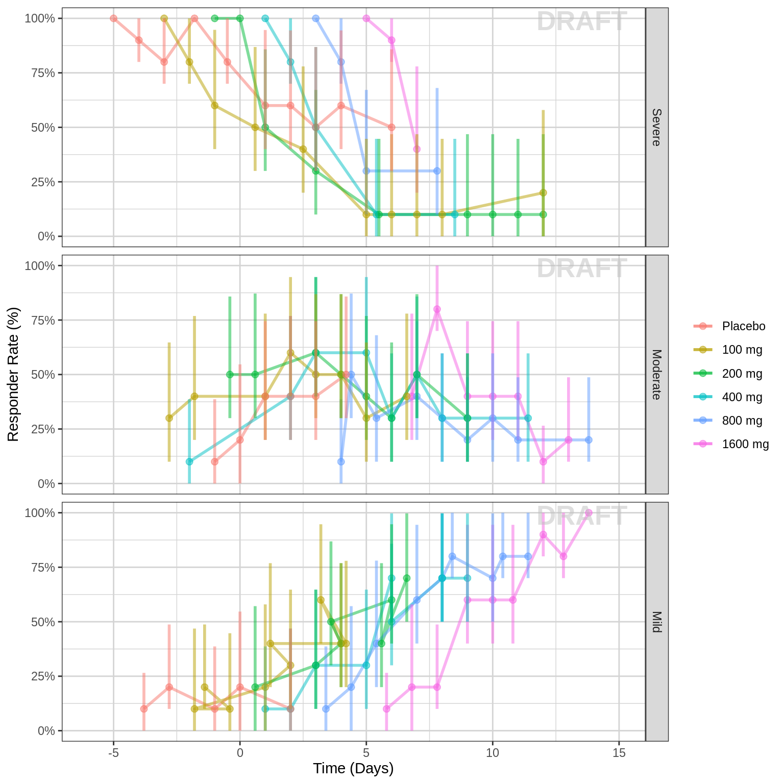
Explore variability
Use spaghetti plots to visualize the extent of variability between individuals. The wider the spread of the profiles, the higher the between subject variability. Distinguish different doses by color, or separate into different panels. If coloring by dose, do the individuals in the different dose groups overlap across doses? Does there seem to be more variability at higher or lower concentrations?
Spaghetti plots of ordinal response over time, faceted by dose
gg <- ggplot(data = pd_data, aes(x = TIME_jitter, y = LIDV_jitter, group = ID))
gg <- gg + xgx_annotate_status(status)
gg <- gg + facet_grid(~TRTACT_low2high)
gg <- gg + geom_line(alpha = 0.5) + geom_point(alpha = 0.5)
gg <- gg + guides(color = guide_legend(""), fill = guide_legend(""))
gg <- gg + xgx_scale_x_time_units(units_dataset = time_units_dataset,
                                  units_plot    = time_units_plot, breaks = seq(0, 8*24, 24))
gg <- gg + labs(y = pd_ordinal_label)
gg <- gg + scale_y_continuous(breaks = c(1, 2, 3), labels = c("Mild", "Moderate", "Severe"))
gg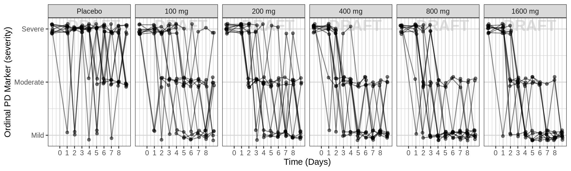
Explore irregularities in profiles
Plot individual profiles in order to inspect them for any irregularities. Inspect the profiles for outlying data points that may skew results or bias conclusions.
Ordinal response over time, faceted by individual, individual line plots
gg <- ggplot(data = pd_data, aes(x = TIME_jitter, y = ORDINAL_LEVELS_low2high))
gg <- gg + xgx_annotate_status(status)
gg <- gg + geom_point( size = 2) +  geom_line( aes(group = ID))
gg <- gg + guides(color = guide_legend(""), fill = guide_legend(""))
gg <- gg + xgx_scale_x_time_units(units_dataset = time_units_dataset,
                                  units_plot    = time_units_plot, breaks = seq(0, 7*24, 7*24))
gg <- gg + facet_wrap(~ID+TRTACT, ncol = length(unique(pd_data$ID))/length(unique(pd_data$DOSE)) )
gg <- gg + labs(y = pd_ordinal_label)
gg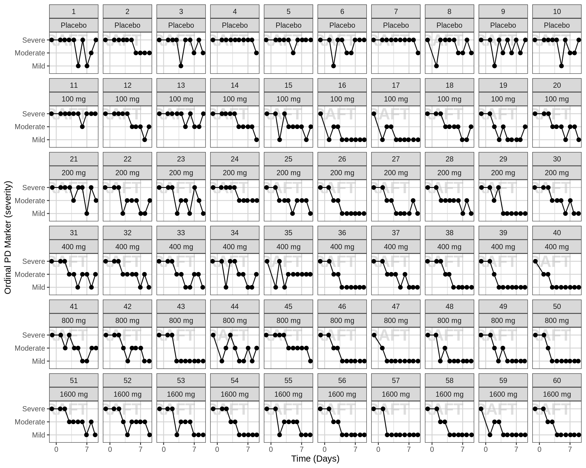
Explore covariate effects on PD
(coming soon)
Explore Dose-Response Relationship
Percent of subjects by response category against dose, at the endpoint of interest
data_to_plot <- pd_data %>% subset(PROFDAY %in% c(SS_PROFDAY), )

gg <- ggplot(data = data_to_plot, aes(x = factor(DOSE), fill = ORDINAL_LEVELS_high2low))
gg <- gg + xgx_annotate_status(status)
gg <- gg + geom_bar(position = "fill") + scale_y_continuous(labels = scales::percent)
gg <- gg + labs(x = dose_label, y = pd_response_label) + guides(fill = guide_legend(""))
gg <- gg + scale_fill_brewer(palette = 6)
gg <- gg + facet_grid(.~DAY_label)

gg2 <- ggplot(data = data_to_plot, aes(x = DOSE, response = ORDINAL_LEVELS_high2low, color = ORDINAL_LEVELS_high2low))
gg2 <- gg2 + xgx_annotate_status(status)
gg2 <- gg2 + xgx_stat_ci(distribution = "ordinal", geom = list("point","errorbar"), position = position_dodge(width = 50))
gg2 <- gg2 + xgx_geom_smooth(method = "polr")
gg2 <- gg2 + scale_y_continuous(labels = scales::percent)
gg2 <- gg2 + labs(x = dose_label, y = pd_response_label) + guides(color = guide_legend(""))
gg2 <- gg2 + facet_grid(.~DAY_label)

grid.arrange(gg, gg2, ncol = 2)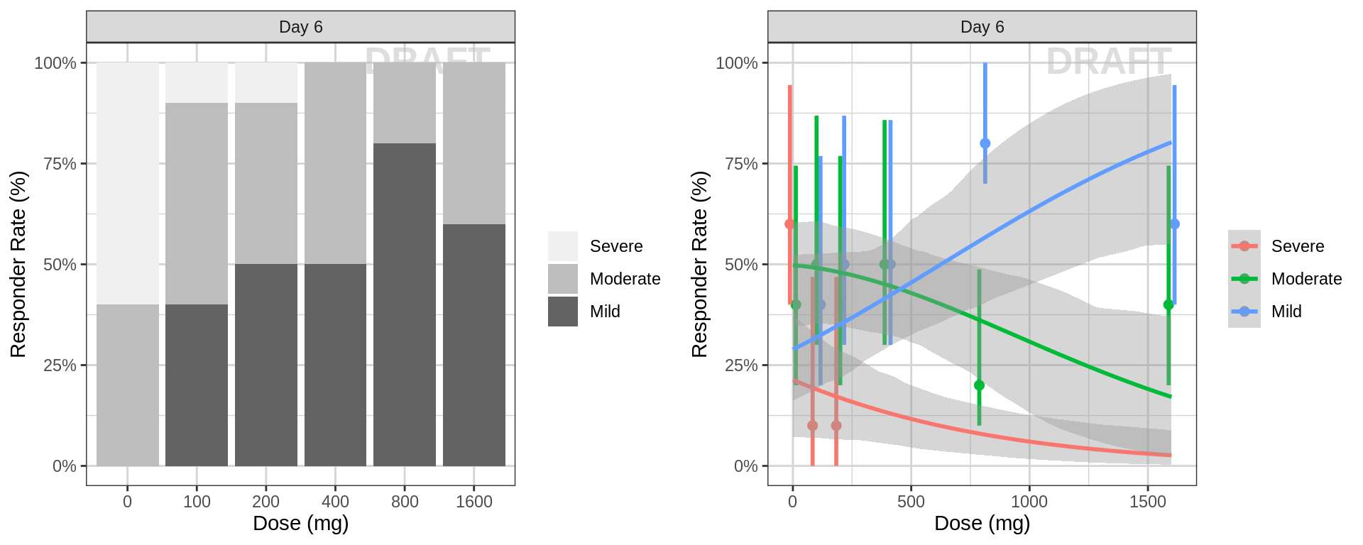
Ordinal response against dose, at the endpoint of interest
data_to_plot <- pd_data %>% subset(PROFDAY %in% c(SS_PROFDAY), )

gg <- ggplot(data = data_to_plot, aes(y = DOSE, x = ORDINAL_LEVELS_low2high))
gg <- gg + geom_jitter(data = data_to_plot,
                       aes(color = TRTACT_high2low), shape = 19, width = 0.1, height = 0, alpha = 0.5)
gg <- gg + xgx_annotate_status(status)
gg <- gg + geom_boxplot(width = 0.5, fill = NA, outlier.shape = NA)
gg <- gg + guides(color = guide_legend(""), fill = guide_legend(""))
gg <- gg + coord_flip()
gg <- gg + labs(y = dose_label, x = pd_ordinal_label)
gg <- gg + facet_grid(.~DAY_label)
gg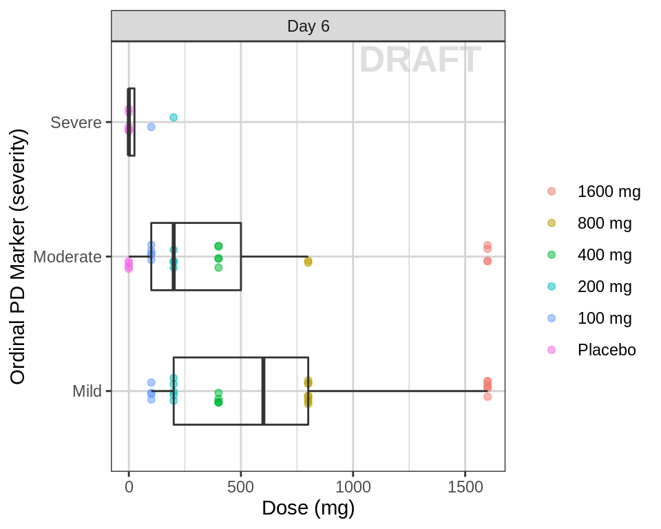
Percent of subjects by response category against dose, faceted by day
data_to_plot <- pd_data %>% subset(PROFDAY %in% PD_PROFDAYS, )

gg <- ggplot(data = data_to_plot, aes(x = factor(DOSE), fill = ORDINAL_LEVELS_high2low))
gg <- gg + xgx_annotate_status(status)
gg <- gg + geom_bar(position = "fill") + scale_y_continuous(labels = scales::percent)
gg <- gg + labs(x = dose_label, y = pd_response_label) + guides(fill = guide_legend(""))
gg <- gg + scale_fill_brewer(palette = 6)
gg <- gg + facet_grid(.~DAY_label)
gg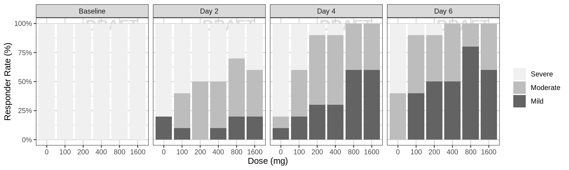
gg <- ggplot(data = data_to_plot, aes(x = DOSE, response = ORDINAL_LEVELS_high2low, color = ORDINAL_LEVELS_high2low))
gg <- gg + xgx_annotate_status(status)
gg <- gg + xgx_stat_ci(distribution = "ordinal", position = position_dodge(width = 50), alpha = 0.5)
gg <- gg + scale_y_continuous(labels = scales::percent)
gg <- gg + labs(x = dose_label, y = pd_response_label) + guides(color = guide_legend(""))
gg <- gg + facet_grid(.~DAY_label)
gg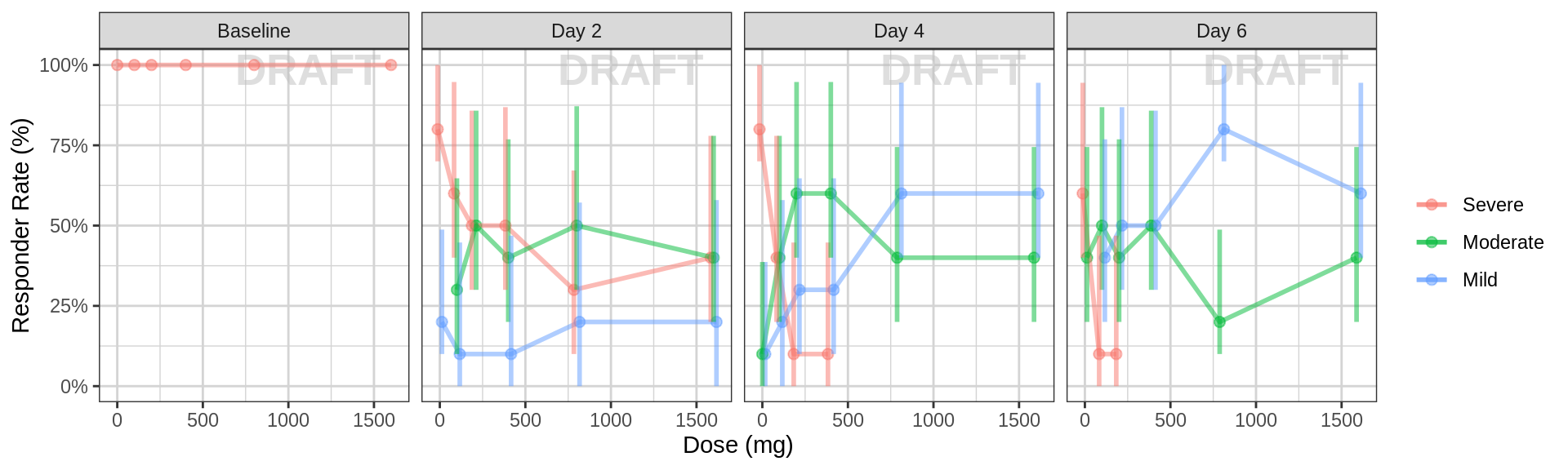
Ordinal response against dose, faceted by day
data_to_plot <- pd_data %>% subset(PROFDAY %in% PD_PROFDAYS, )

gg <- ggplot(data = data_to_plot, aes(y = DOSE, x = ORDINAL_LEVELS_low2high))+theme_bw()
gg <- gg + geom_jitter(data = data_to_plot,
                       aes(color = TRTACT), shape = 19, width = 0.1, height = 0, alpha = 0.5)
gg <- gg + xgx_annotate_status(status)
gg <- gg + geom_boxplot(width = 0.5, fill = NA, outlier.shape = NA)
gg <- gg + guides(color = guide_legend(""), fill = guide_legend(""))
gg <- gg + coord_flip()
gg <- gg + xlab(pd_ordinal_label) + ylab("Dose (mg)")
gg <- gg + facet_grid(.~DAY_label)
gg <- gg + labs(y = dose_label, x = pd_ordinal_label)
gg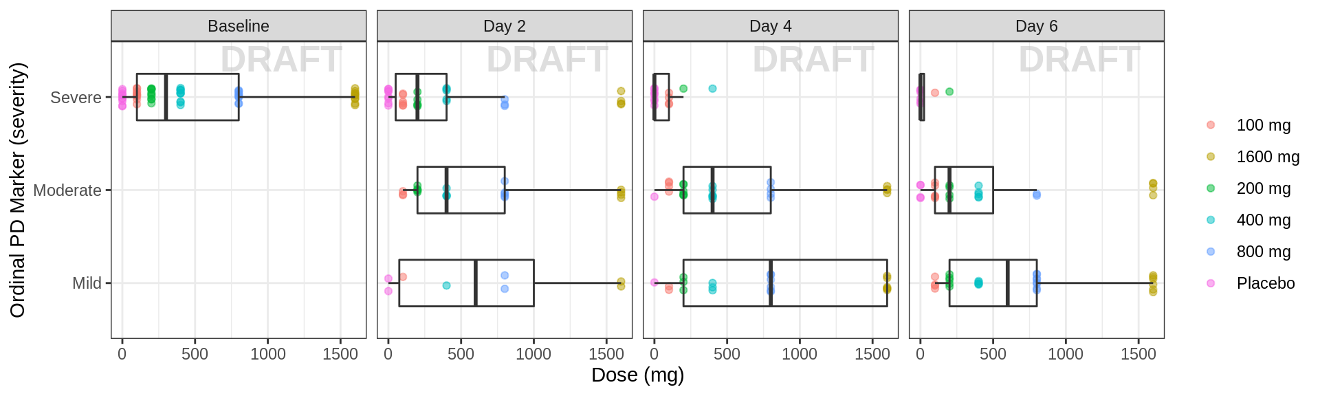
R Session Info
sessionInfo()## R version 4.1.0 (2021-05-18)
## Platform: x86_64-pc-linux-gnu (64-bit)
## Running under: Red Hat Enterprise Linux Server 7.9 (Maipo)
##
## Matrix products: default
## BLAS/LAPACK: /CHBS/apps/EB/software/imkl/2019.1.144-gompi-2019a/compilers_and_libraries_2019.1.144/linux/mkl/lib/intel64_lin/libmkl_gf_lp64.so
##
## locale:
## [1] LC_CTYPE=en_US.UTF-8 LC_NUMERIC=C LC_TIME=en_US.UTF-8 LC_COLLATE=en_US.UTF-8 LC_MONETARY=en_US.UTF-8
## [6] LC_MESSAGES=en_US.UTF-8 LC_PAPER=en_US.UTF-8 LC_NAME=C LC_ADDRESS=C LC_TELEPHONE=C
## [11] LC_MEASUREMENT=en_US.UTF-8 LC_IDENTIFICATION=C
##
## attached base packages:
## [1] stats graphics grDevices utils datasets methods base
##
## other attached packages:
## [1] DT_0.26 forcats_0.5.2 stringr_1.4.1 purrr_0.3.5 readr_2.1.3 tibble_3.1.8 tidyverse_1.3.2 xgxr_1.1.1 zoo_1.8-11
## [10] gridExtra_2.3 tidyr_1.2.1 dplyr_1.0.10 ggplot2_3.3.6
##
## loaded via a namespace (and not attached):
## [1] googledrive_2.0.0 colorspace_2.0-3 deldir_1.0-6 ellipsis_0.3.2 class_7.3-19 htmlTable_2.2.1 markdown_1.2
## [8] base64enc_0.1-3 fs_1.5.2 gld_2.6.2 rstudioapi_0.14 proxy_0.4-26 farver_2.1.1 Deriv_4.1.3
## [15] fansi_1.0.3 mvtnorm_1.1-3 lubridate_1.8.0 xml2_1.3.3 codetools_0.2-18 splines_4.1.0 cachem_1.0.6
## [22] rootSolve_1.8.2.2 knitr_1.40 Formula_1.2-4 jsonlite_1.8.3 broom_1.0.1 binom_1.1-1 cluster_2.1.3
## [29] dbplyr_2.2.1 png_0.1-7 compiler_4.1.0 httr_1.4.4 backports_1.4.1 assertthat_0.2.1 Matrix_1.5-1
## [36] fastmap_1.1.0 gargle_1.2.1 cli_3.4.1 prettyunits_1.1.1 htmltools_0.5.3 tools_4.1.0 gtable_0.3.1
## [43] glue_1.6.2 lmom_2.8 Rcpp_1.0.9 cellranger_1.1.0 jquerylib_0.1.4 vctrs_0.5.0 nlme_3.1-160
## [50] crosstalk_1.2.0 xfun_0.34 rvest_1.0.3 lifecycle_1.0.3 googlesheets4_1.0.1 MASS_7.3-58.1 scales_1.2.1
## [57] hms_1.1.2 expm_0.999-6 RColorBrewer_1.1-3 yaml_2.3.6 Exact_2.1 pander_0.6.4 sass_0.4.2
## [64] rpart_4.1.16 reshape_0.8.8 latticeExtra_0.6-30 stringi_1.7.8 highr_0.9 e1071_1.7-8 checkmate_2.1.0
## [71] boot_1.3-28 rlang_1.0.6 pkgconfig_2.0.3 bitops_1.0-7 evaluate_0.17 lattice_0.20-45 htmlwidgets_1.5.4
## [78] labeling_0.4.2 tidyselect_1.2.0 GGally_2.1.2 plyr_1.8.7 magrittr_2.0.3 R6_2.5.1 DescTools_0.99.42
## [85] generics_0.1.3 Hmisc_4.7-0 DBI_1.1.3 pillar_1.8.1 haven_2.5.1 foreign_0.8-82 withr_2.5.0
## [92] mgcv_1.8-41 survival_3.4-0 RCurl_1.98-1.4 nnet_7.3-17 crayon_1.5.2 modelr_0.1.9 interp_1.1-2
## [99] utf8_1.2.2 tzdb_0.3.0 rmarkdown_2.17 progress_1.2.2 jpeg_0.1-9 grid_4.1.0 readxl_1.4.1
## [106] minpack.lm_1.2-1 data.table_1.14.2 reprex_2.0.2 digest_0.6.30 munsell_0.5.0 bslib_0.4.0