Overview
tinydenseR is a landmark-based platform for single cell data analysis that identifies differential cell states and features, including subtle within-cluster state changes. Modeling samples as replicates, tinydenseR enhances analytic efficiency and reproducibility while preserving the richness of single cell data.
Why use tinydenseR? Traditional single-cell analysis methods rely heavily on clustering, which can be oversimplified and subjective. tinydenseR provides a clustering-independent framework that preserves biological complexity while maintaining statistical rigor.
For details, check out our preprint on bioRxiv!

Key Features
- 🎯 Sample-centric analysis: Treats samples, not cells, as biological replicates for proper statistical modeling
-
🚀 Memory efficient: Handles atlas-scale datasets with minimal memory footprint
- 🔬 Multi-technology support: Works with scRNA-seq, flow cytometry, mass cytometry (multi-modal data support coming soon)
- 📊 Rich visualizations: Built-in plotting functions for exploring results
- 🔗 Clinical integration: Links cell-level variation to clinical and experimental outcomes
- ⚡ Fast processing: Efficient algorithms for large-scale data analysis
Installation
Dependencies
tinydenseR requires R (>= 4.1) and Bioconductor and CRAN packages. Most dependencies will be installed automatically, but you may need to install some of them manually, like BPCells:
#install_github()` was deprecated in devtools 2.5.0
if (!require("pak")) install.packages("pak")
pak::pkg_install(pkg = "Novartis/tinydenseR")
# pak::pkg_install(pkg = "bnprks/BPCells/r")
Example
This example demonstrates the tinydenseR workflow on a synthetic scRNA-seq trajectory dataset with two conditions (A and B) and three replicates per condition (5,000 cells, 500 genes). Condition effects are introduced by systematically varying the proportion of cells assigned to each condition at each trajectory milestone, creating differential cell-state abundance along the trajectory.
Build Landmarks with RunTDR()
RunTDR() selects landmark cells, builds a nearest-neighbor graph, clusters landmarks, maps all cells to their nearest landmarks to generate the landmark-by-sample matrix in a single call. Unsupervised sample embedding is also returned automatically.
sim_trajectory <-
  tinydenseR::RunTDR(
    x = sim_trajectory,
    .sample.var = "Sample",
    .assay.type = "RNA",
    .nHVG = 500,
    .verbose = FALSE,
    .seed = 123 # for reproducibility
  )
#> Loading required namespace: SingleCellExperiment
#> Warning in (function (A, nv = 5, nu = nv, maxit = 1000, work = nv + 7, reorth =
#> TRUE, : You're computing too large a percentage of total singular values, use a
#> standard svd instead.
Differential Density Analysis with get.lm()
We set up a design matrix and test which landmarks show differential density between conditions.
.design <-
  model.matrix(~ Condition,
               data = tinydenseR::GetTDR(sim_trajectory)@metadata)

sim_trajectory <-
  tinydenseR::get.lm(
    x = sim_trajectory,
    .design = .design,
    .verbose = FALSE
  )
#> Warning in get.lm.TDRObj(tdr, ...): PCA-weighted q-value estimation is not
#> recommended for fewer than 1000 tests. Using standard q-value estimation
#> instead.
#> Warning in value[[3L]](cond): q-value estimation failed. Using BH instead.
#> Warning in get.lm.TDRObj(tdr, ...): Only 1 cluster detected. Skipping limma fit
#> on cluster composition (nothing to compare). Density-level analysis (get.plsD,
#> get.dea, etc.) is unaffected.
Sample Embedding
We fit a reduced (intercept-only) model and compute partial-effect PCs to produce a quantitative per-sample score along the Condition axis.
# Reduced model (no Condition term)
noCondition.design <-
  model.matrix(~ 1,
               data = tinydenseR::GetTDR(sim_trajectory)@metadata)

sim_trajectory <-
  tinydenseR::get.lm(
    x = sim_trajectory,
    .design = noCondition.design,
    .model.name = "noCondition",
    .verbose = FALSE
  )
#> Warning in get.lm.TDRObj(tdr, ...): PCA-weighted q-value estimation is not
#> recommended for fewer than 1000 tests. Using standard q-value estimation
#> instead.
#> Warning in get.lm.TDRObj(tdr, ...): Only 1 cluster detected. Skipping limma fit
#> on cluster composition (nothing to compare). Density-level analysis (get.plsD,
#> get.dea, etc.) is unaffected.

# Compute partial-effect PCs
sim_trajectory <-
  tinydenseR::get.embedding(
    x = sim_trajectory,
    .full.model = "default",
    .red.model = "noCondition",
    .term.of.interest = "Condition",
    .verbose = FALSE
  )
# Unsupervised sample PCA
smpl.pca <-
  tinydenseR::plotSampleEmbedding(
    x = sim_trajectory,
    .embedding = "pca",
    .color.by = "Condition",
    .cat.feature.color = tinydenseR::Color.Palette[1, c(1, 2)],
    .panel.size = 1.5,
    .point.size = 3
  ) +
  ggplot2::labs(title = "PCA") +
  ggplot2::theme(plot.title = ggplot2::element_text(hjust = 0.5),
                 legend.position = "bottom")

# Supervised partial-effect PC
smpl.pePC <-
  tinydenseR::plotSampleEmbedding(
    x = sim_trajectory,
    .embedding = "pePC",
    .sup.embed.slot = "Condition",
    .color.by = "Condition",
    .cat.feature.color = tinydenseR::Color.Palette[1, c(1, 2)],
    .panel.size = 1.5,
    .point.size = 3
  ) +
  ggplot2::labs(title = "partial-effect PC") +
  ggplot2::theme(plot.title = ggplot2::element_text(hjust = 0.5),
                 legend.position = "bottom")

(smpl.pca | smpl.pePC) +
  patchwork::plot_layout(guides = "collect") &
  ggplot2::theme(legend.position = "bottom",
                 legend.justification = "center")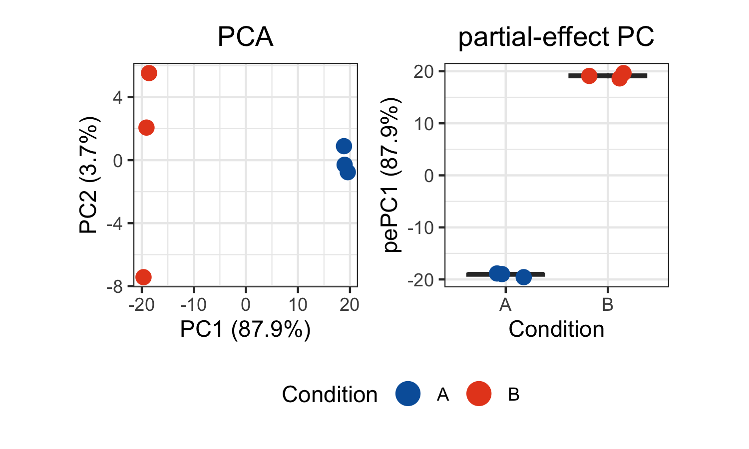
The unsupervised PCA shows inter-sample variation based on density profiles across landmarks. The supervised partial-effect PC isolates variation along the Condition axis, clearly separating the two groups.
Density Contrast and plsD
We decompose the density contrast into interpretable gene-expression programs using get.plsD(), and visualize the result as a patchwork of the density fold-change and plsD1 scores on the landmark PCA.
sim_trajectory <-
  tinydenseR::get.plsD(
    x = sim_trajectory,
    .coef.col = "ConditionB",
    .model.name = "default",
    .verbose = FALSE
  )
# Density fold-change on landmark PCA
dens.p <-
  tinydenseR::plotPCA(
    x = sim_trajectory,
    .feature = tinydenseR::GetTDR(sim_trajectory)@results$lm$default$fit$coefficients[, "ConditionB"],
    .panel.size = 1.5,
    .point.size = 1,
    .color.label = "density\nlog2(+0.5)FC",
    .midpoint = 0,
    .legend.position = "bottom"
  ) +
  ggplot2::guides(color = ggplot2::guide_colorbar(title.position = "top",
                                                  title.hjust = 0.5)) +
  ggplot2::theme(plot.subtitle = ggplot2::element_blank(),
                 legend.margin = ggplot2::margin(t = -0.1, unit = "in"))

# plsD1 scores on landmark PCA
plsD1.p <-
  tinydenseR::plotPlsD(
    x = sim_trajectory,
    .coef.col = "ConditionB",
    .plsD.dim = 1,
    .embed = "pca",
    .panel.size = 1.5
  )[[1]]

# Patchwork: density contrast | plsD1
((dens.p +
    ggplot2::labs(title = "") +
    ggplot2::theme(legend.margin = ggplot2::margin(t = -0.1,
                                                   unit = "in"))) |
   (plsD1.p +
      ggplot2::labs(title = "") +
      ggplot2::theme(legend.margin = ggplot2::margin(t = 0.1,
                                                     unit = "in")))) +
  patchwork::plot_annotation(title = "Density contrast: Condition B vs A") &
  ggplot2::theme(
    plot.title =
      ggplot2::element_text(hjust = 0.5,
                            margin = ggplot2::margin(t = -0.1,
                                                     unit = "in")))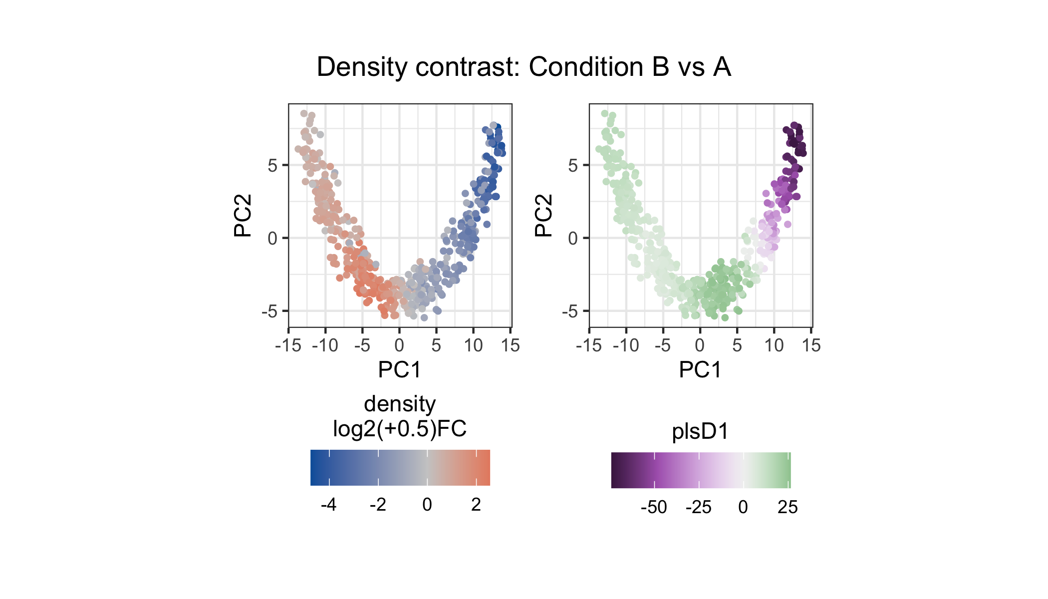
The left panel shows density log2 fold-change at each landmark: landmarks enriched in Condition B are red, those enriched in A are blue. The right panel shows plsD1 scores, which capture the leading gene-expression program aligned with the density contrast.
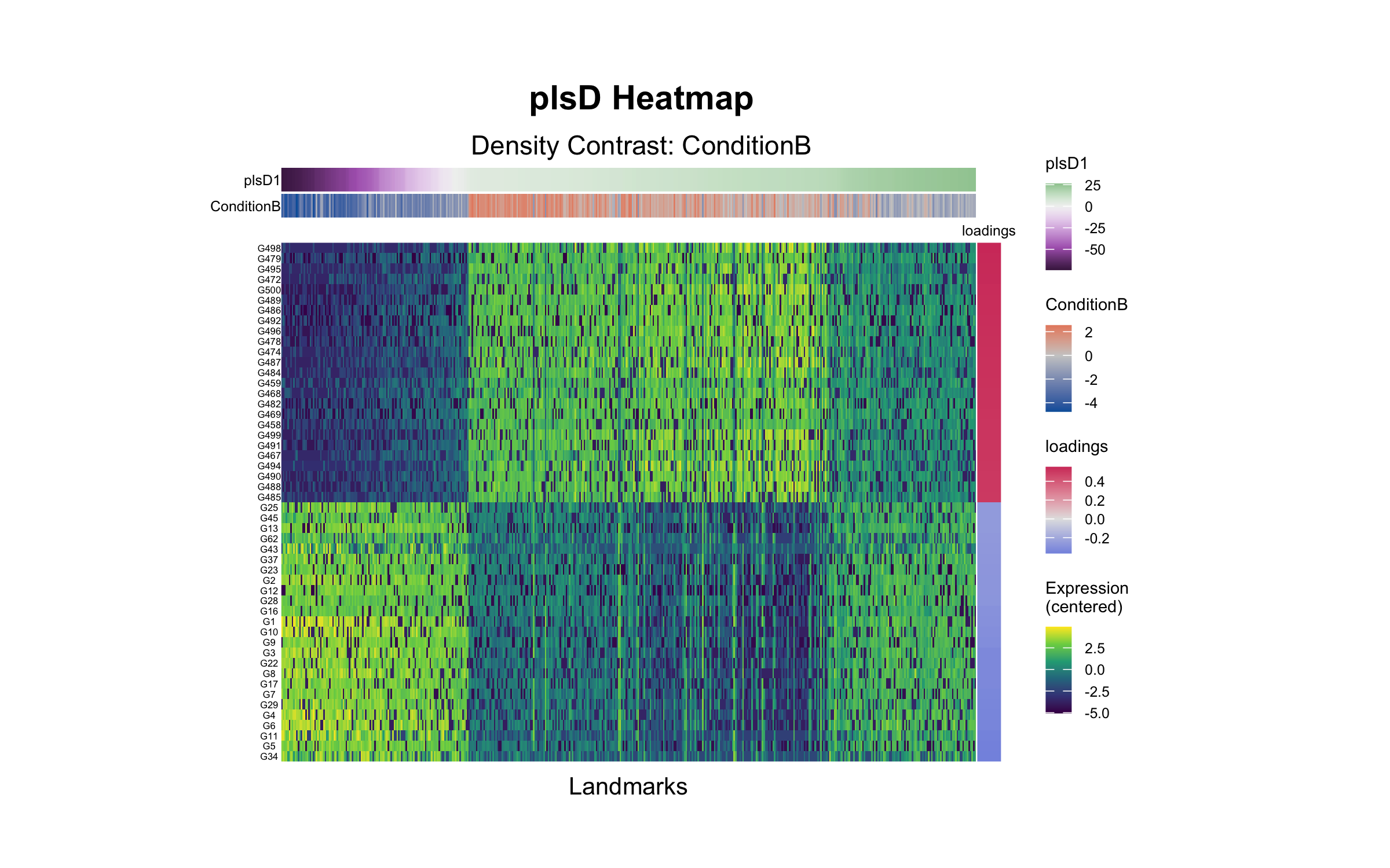
plsD Heatmap
The plsD heatmap shows landmark expression profiles ordered by plsD1 scores, with gene loadings on the right. Rows display centered expression of the top 25 features associated with each direction of plsD1.
tinydenseR::plotPlsDHeatmap(
  x = sim_trajectory,
  .coef.col = "ConditionB",
  .plsD.dim = 1,
  .order.by = "plsD.dim",
  .panel.height = 3,
  .feature.font.size = 4
)
tinydenseR recovered trajectory-associated cell-state changes, embedded samples along the variable of interest, and uncovered gene-expression programs associated with changes in cell density, illustrating its ability to model continuous cellular and molecular variation without relying on hard cluster boundaries.
Getting Help
Documentation
Function documentation: Use
?function_namein R for detailed help on any functionReproducible scripts: Check the
inst/scripts/directory for example workflows
Troubleshooting Common Issues
Installation problems:
Ensure you have R >= 4.1
Install BiocManager first:
install.packages("BiocManager")Try installing dependencies manually if automatic installation fails
Questions and Support:
🐛 Report bugs: GitHub Issues
💬 Discussions: Use GitHub Discussions for general questions
Contributing
We welcome contributions to tinydenseR! Here’s how you can help:
License
The code is licensed under the MIT License (see LICENSE.md).
The sticker artwork (PNG) is licensed under CC0 (see LICENSE-artwork).
Copyright 2025 Novartis Biomedical Research Inc.